Built using Zelig version 5.1.4.90000

Zelig workflow overview

All models in Zelig can be estimated and results explored presented using four simple functions:

1. zelig to estimate the parameters,

2. setx to set fitted values for which we want to find quantities of interest,

3. sim to simulate the quantities of interest,

4. plot to plot the simulation results.

Zelig 5 reference classes

Zelig 5 introduced reference classes. These enable a different way of working with Zelig that is detailed in a separate vignette. Directly using the reference class architecture is optional.

Examples

Let’s walk through an example. This example uses the swiss dataset. It contains data on fertility and socioeconomic factors in Switzerland’s 47 French-speaking provinces in 1888 (Mosteller and Tukey, 1977, 549-551). We will model the effect of education on fertility, where education is measured as the percent of draftees with education beyond primary school and fertility is measured using the common standardized fertility measure (see Muehlenbein (2010, 80-81) for details).

Installing and Loading Zelig

If you haven’t already done so, open your R console and install Zelig. We recommend installing Zelig with the zeligverse package. This installs core Zelig and ancillary packages at once.

install.packages('zeligverse')

Alternatively you can install the development version of Zelig with:

devtools::install_github('IQSS/Zelig')

Once Zelig is installed, load it:

library(zeligverse)

Building Models

Let’s assume we want to estimate the effect of education on fertility. Since fertility is a continuous variable, least squares (ls) is an appropriate model choice. To estimate our model, we call the zelig() function with three two arguments: equation, model type, and data:

# load data
data(swiss)

# estimate ls model
z5_1 <- zelig(Fertility ~ Education, model = "ls", data = swiss, cite = FALSE)

# model summary
summary(z5_1)

## Model: 
## 
## Call:
## z5$zelig(formula = Fertility ~ Education, data = swiss)
## 
## Residuals:
##     Min      1Q  Median      3Q     Max 
## -17.036  -6.711  -1.011   9.526  19.689 
## 
## Coefficients:
##             Estimate Std. Error t value Pr(>|t|)
## (Intercept)  79.6101     2.1041  37.836  < 2e-16
## Education    -0.8624     0.1448  -5.954 3.66e-07
## 
## Residual standard error: 9.446 on 45 degrees of freedom
## Multiple R-squared:  0.4406, Adjusted R-squared:  0.4282 
## F-statistic: 35.45 on 1 and 45 DF,  p-value: 3.659e-07
## 
## Next step: Use 'setx' method

The -0.86 coefficient on education suggests a negative relationship between the education of a province and its fertility rate. More precisely, for every one percent increase in draftees educated beyond primary school, the fertility rate of the province decreases 0.86 units. To help us better interpret this finding, we may want other quantities of interest, such as expected values or first differences. Zelig makes this simple by automating the translation of model estimates into interpretable quantities of interest using Monte Carlo simulation methods (see King, Tomz, and Wittenberg (2000) for more information). For example, let’s say we want to examine the effect of increasing the percent of draftees educated from 5 to 15. To do so, we set our predictor value using the setx() and setx1() functions:

# set education to 5 and 15
z5_1 <- setx(z5_1, Education = 5)
z5_1 <- setx1(z5_1, Education = 15)

# model summary
summary(z5_1)

## setx:
##   (Intercept) Education
## 1           1         5
## setx1:
##   (Intercept) Education
## 1           1        15
## 
## Next step: Use 'sim' method

After setting our predictor value, we simulate using the sim() method:

# run simulations and estimate quantities of interest
z5_1 <- sim(z5_1)

# model summary
summary(z5_1)

## 
##  sim x :
##  -----
## ev
##       mean       sd      50%     2.5%   97.5%
## 1 75.33601 1.568926 75.35504 71.98253 78.3214
## pv
##          mean       sd      50%    2.5%    97.5%
## [1,] 75.71558 9.525293 75.73353 58.5333 95.91194
## 
##  sim x1 :
##  -----
## ev
##       mean       sd      50%     2.5%   97.5%
## 1 66.71969 1.454155 66.67102 63.87779 69.5769
## pv
##          mean       sd      50%     2.5%    97.5%
## [1,] 66.87073 9.578544 66.88007 48.02027 84.90856
## fd
##        mean       sd       50%      2.5%     97.5%
## 1 -8.616321 1.416013 -8.591192 -11.34729 -5.964767

At this point, we’ve estimated a model, set the predictor value, and estimated easily interpretable quantities of interest. The summary() method shows us our quantities of interest, namely, our expected and predicted values at each level of education, as well as our first differences–the difference in expected values at the set levels of education.

Visualizations

Zelig’s plot() function plots the estimated quantities of interest:

plot(z5_1)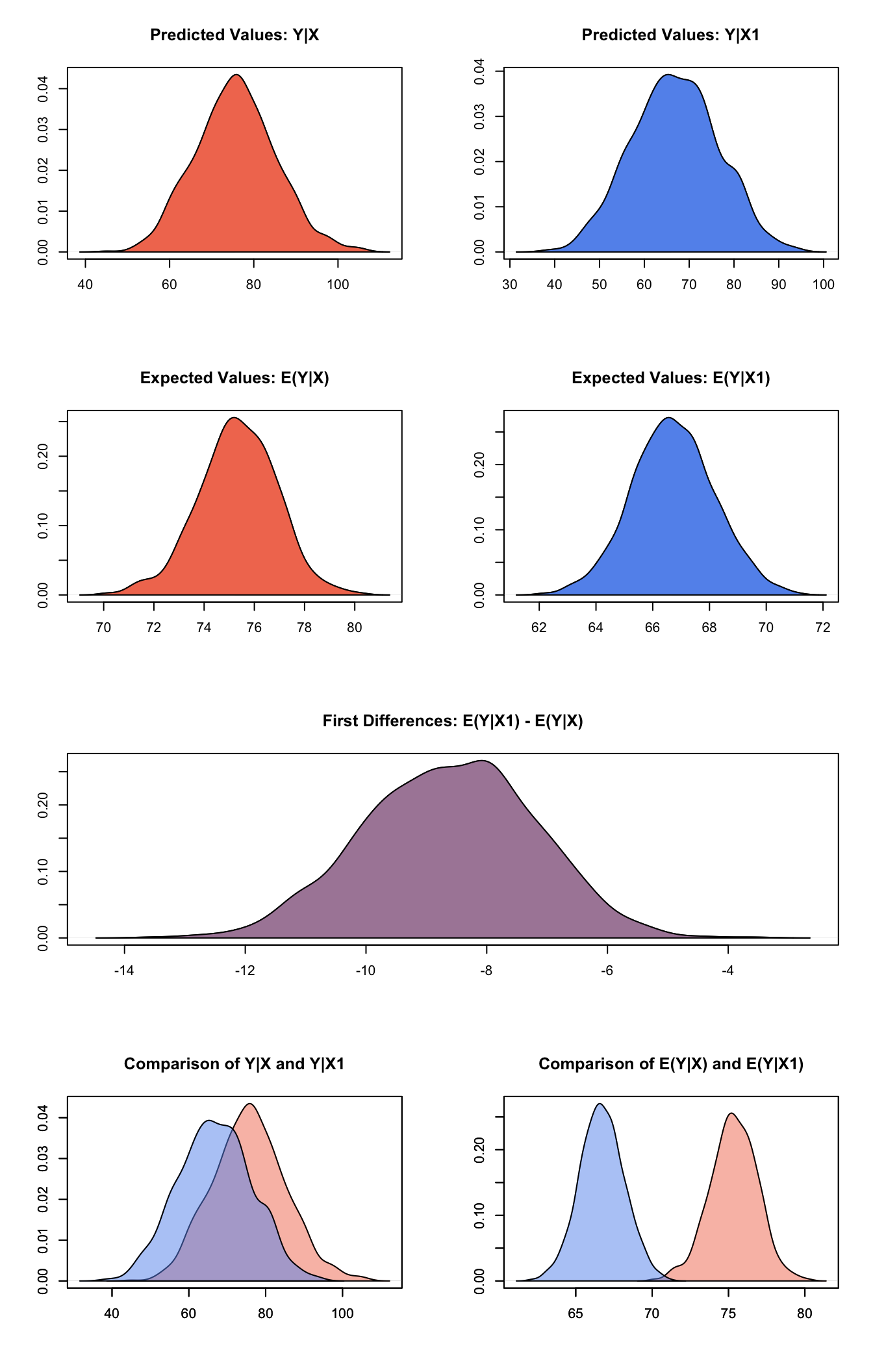

We can also simulate and plot simulations from ranges of simulated values:

z5_2 <- zelig(Fertility ~ Education, model = "ls", data = swiss, cite = FALSE)

# set Education to range from 5 to 15 at single integer increments
z5_2 <- setx(z5_2, Education = 5:15)

# run simulations and estimate quantities of interest
z5_2 <- sim(z5_2)

Then use the plot() function as before:

z5_2 <- plot(z5_2)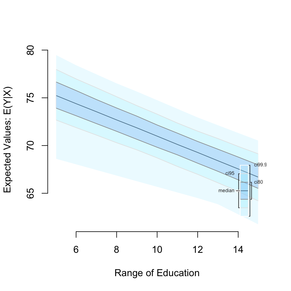

Getting help

The primary documentation for Zelig is available at: http://docs.zeligproject.org/articles/.

Within R, you can access function help using the normal ? function, e.g.:

?setx

If you are looking for details on particlar estimation model methods, you can also use the ? function. Simply place a z before the model name. For example, to access details about the logit model use:

?zlogit