Logit GEE

Built using Zelig version 5.1.4.90000

Generalized Estimating Equation for Logit Regression with logit.gee.

The GEE logit estimates the same model as the standard logit regression (appropriate when you have a dichotomous dependent variable and a set of explanatory variables). Unlike in logit regression, GEE logit allows for dependence within clusters, such as in longitudinal data, although its use is not limited to just panel data. The user must first specify a “working” correlation matrix for the clusters, which models the dependence of each observation with other observations in the same cluster. The “working” correlation matrix is a $T \times T$ matrix of correlations, where $T$ is the size of the largest cluster and the elements of the matrix are correlations between within-cluster observations. The appeal of GEE models is that it gives consistent estimates of the parameters and consistent estimates of the standard errors can be obtained using a robust “sandwich” estimator even if the “working” correlation matrix is incorrectly specified. If the “working” correlation matrix is correctly specified, GEE models will give more efficient estimates of the parameters. GEE models measure population-averaged effects as opposed to cluster-specific effects.

Syntax

z.out <- zelig(Y ~ X1 + X2, model = "logit.gee",
               id = "X3", weights = w, data = mydata)
x.out <- setx(z.out)
s.out <- sim(z.out, x = x.out)

where id is a variable which identifies the clusters. The data should be sorted by id and should be ordered within each cluster when appropriate.

Additional Inputs

Use the following arguments to specify the structure of the “working” correlations within clusters:

corstr: character string specifying the correlation structure: “independence”, “exchangeable”, “ar1”, “unstructured” and “userdefined”
See geeglm in package geepack for other function arguments.

Examples

Example with Stationary 3 Dependence

Attaching the sample turnout dataset:

data(turnout)

Variable identifying clusters

turnout$cluster <- rep(c(1:200), 10)
sorted.turnout <- turnout[order(turnout$cluster),]

Estimating parameter values:

z.out1 <- zelig(vote ~ race + educate, model = "logit.gee",
                id = "cluster", data = sorted.turnout)

## How to cite this model in Zelig:
##   Patrick Lam. 2011.
##   logit-gee: General Estimating Equation for Logistic Regression
##   in Christine Choirat, Christopher Gandrud, James Honaker, Kosuke Imai, Gary King, and Olivia Lau,
##   "Zelig: Everyone's Statistical Software," http://zeligproject.org/

summary(z.out1)

## Model: 
## 
## Call:
## z5$zelig(formula = vote ~ race + educate, id = "cluster", data = sorted.turnout)
## 
##  Coefficients:
##             Estimate  Std.err  Wald Pr(>|W|)
## (Intercept) -1.21890  0.21897 30.99  2.6e-08
## racewhite    0.50223  0.14108 12.67 0.000371
## educate      0.16100  0.01621 98.61  < 2e-16
## 
## Estimated Scale Parameters:
##             Estimate Std.err
## (Intercept)   0.9833 0.04661
## 
## Correlation: Structure = independenceNumber of clusters:   200   Maximum cluster size: 10 
## Next step: Use 'setx' method

Setting values for the explanatory variables to their default values:

x.out1 <- setx(z.out1)

Simulating quantities of interest:

s.out1 <- sim(z.out1, x = x.out1)

summary(s.out1)

## 
##  sim x :
##  -----
## ev
##        mean      sd    50%   2.5%  97.5%
## [1,] 0.7727 0.01132 0.7734 0.7506 0.7939
## pv
##          0     1
## [1,] 0.225 0.775

plot(s.out1)

Graphs of Quantities of Interest for Zelig-logitgee1

Simulating First Differences

Estimating the risk difference (and risk ratio) between low education (25th percentile) and high education (75th percentile) while all the other variables held at their default values.

x.high <- setx(z.out1, educate = quantile(turnout$educate, prob = 0.75))
x.low <- setx(z.out1, educate = quantile(turnout$educate, prob = 0.25))

s.out2 <- sim(z.out1, x = x.high, x1 = x.low)

summary(s.out2)

## 
##  sim x :
##  -----
## ev
##        mean      sd    50%   2.5%  97.5%
## [1,] 0.8232 0.01056 0.8237 0.8018 0.8434
## pv
##          0     1
## [1,] 0.183 0.817
## 
##  sim x1 :
##  -----
## ev
##        mean     sd    50%   2.5%  97.5%
## [1,] 0.7094 0.0146 0.7091 0.6805 0.7372
## pv
##          0     1
## [1,] 0.282 0.718
## fd
##         mean      sd    50%   2.5%    97.5%
## [1,] -0.1139 0.01207 -0.114 -0.136 -0.09029

plot(s.out2)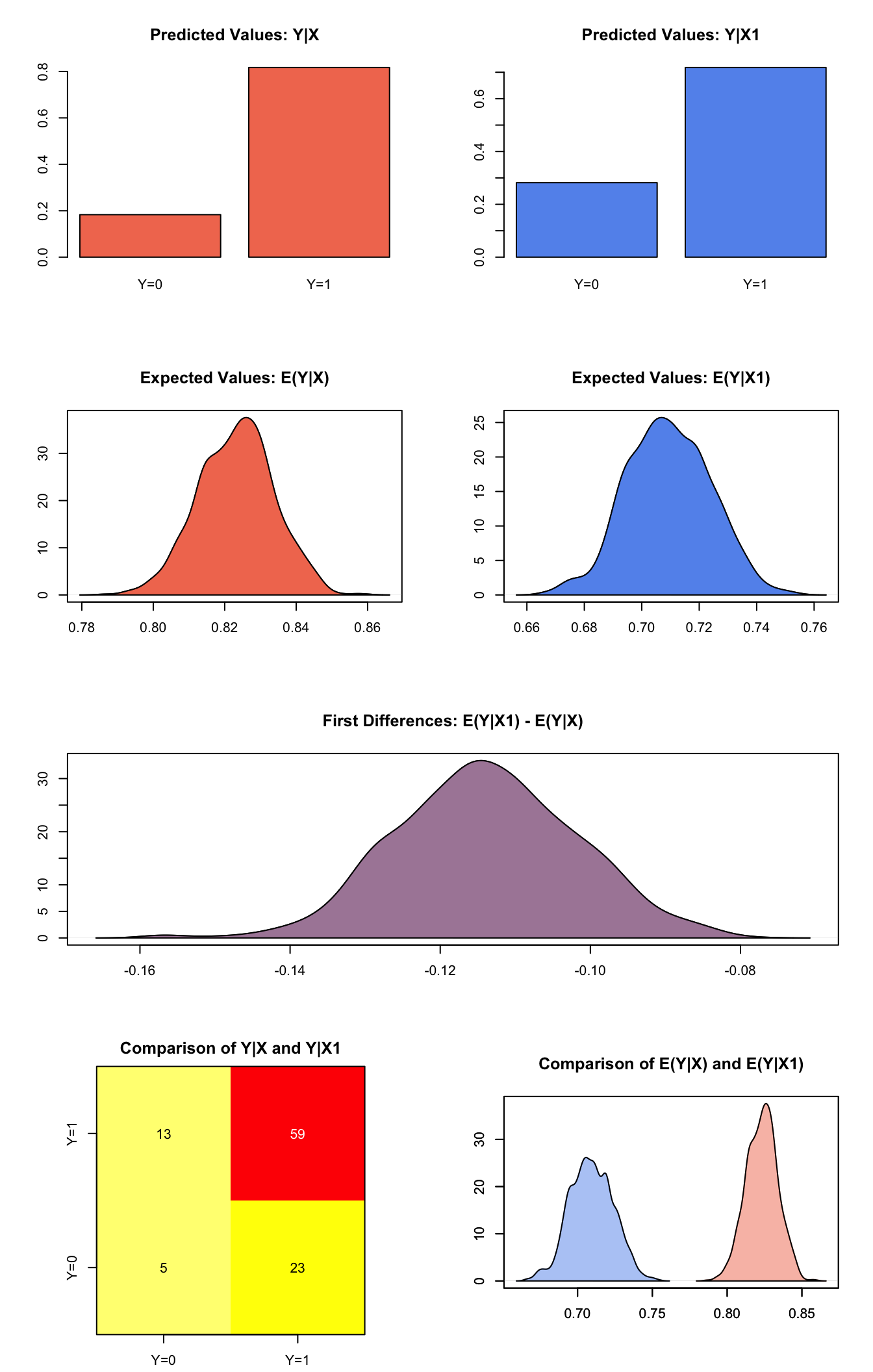

Graphs of Quantities of Interest for Zelig-logitgee2

Example with Fixed Correlation Structure

User-defined correlation structure

library(geepack)

corr.mat <- matrix(rep(0.5, 100), nrow = 10, ncol = 10)
diag(corr.mat) <- 1
corr.mat <- fixed2Zcor(corr.mat, id = sorted.turnout$cluster,
                       waves = sorted.turnout$race)

Generating empirical estimates:

z.out2 <- zelig(vote ~ race + educate, model = "logit.gee",
                id = "cluster", data = sorted.turnout,
                corstr = "fixed", zcor = corr.mat)

## How to cite this model in Zelig:
##   Patrick Lam. 2011.
##   logit-gee: General Estimating Equation for Logistic Regression
##   in Christine Choirat, Christopher Gandrud, James Honaker, Kosuke Imai, Gary King, and Olivia Lau,
##   "Zelig: Everyone's Statistical Software," http://zeligproject.org/

Viewing the regression output:

summary(z.out2)

## Model: 
## 
## Call:
## z5$zelig(formula = vote ~ race + educate, id = "cluster", zcor = corr.mat, 
##     corstr = "fixed", data = sorted.turnout)
## 
##  Coefficients:
##             Estimate Std.err Wald Pr(>|W|)
## (Intercept)   -1.219   0.000  Inf   <2e-16
## racewhite      0.502   0.000  Inf   <2e-16
## educate        0.161   0.000  Inf   <2e-16
## 
## Estimated Scale Parameters:
##             Estimate Std.err
## (Intercept)    0.983  0.0325
## 
## Correlation: Structure = fixed  Link = identity 
## 
## Estimated Correlation Parameters:
##         Estimate Std.err
## alpha:1        1       0
## Number of clusters:   200   Maximum cluster size: 10 
## Next step: Use 'setx' method

The Model

Suppose we have a panel dataset, with $Y_{it}$ denoting the binary dependent variable for unit $i$ at time $t$. $Y_{i}$ is a vector or cluster of correlated data where $y_{it}$ is correlated with $y_{it^\prime}$ for some or all $t, t^\prime$. Note that the model assumes correlations within $i$ but independence across $i$.

The stochastic component is given by the joint and marginal distributions

\[ \begin{aligned} Y_{i} &\sim& f(y_{i} \mid \pi_{i})\\ Y_{it} &\sim& g(y_{it} \mid \pi_{it})\end{aligned} \] where $f$ and $g$ are unspecified distributions with means $\pi_{i}$ and $\pi_{it}$. GEE models make no distributional assumptions and only require three specifications: a mean function, a variance function, and a correlation structure.

The systematic component is the mean function, given by:

\[ \pi_{it} = \Phi(x_{it} \beta) \]

where $\Phi(\mu)$ is the cumulative distribution function of the Normal distribution with mean 0 and unit variance, $x_{it}$ is the vector of $k$ explanatory variables for unit $i$ at time $t$ and $\beta$ is the vector of coefficients.

The variance function is given by:

\[ V_{it} = \pi_{it} (1-\pi_{it}) \]

The correlation structure is defined by a $T \times T$ “working” correlation matrix, where $T$ is the size of the largest cluster. Users must specify the structure of the “working” correlation matrix a priori. The “working” correlation matrix then enters the variance term for each $i$, given by:

\[ V_{i} = \phi \, A_{i}^{\frac{1}{2}} R_{i}(\alpha) A_{i}^{\frac{1}{2}} \]

where $A_{i}$ is a $T \times T$ diagonal matrix with the variance function $V_{it} = \pi_{it} (1-\pi_{it})$ as the $t$ th diagonal element, $R_{i}(\alpha)$ is the “working” correlation matrix, and $\phi$ is a scale parameter. The parameters are then estimated via a quasi-likelihood approach.

In GEE models, if the mean is correctly specified, but the variance and correlation structure are incorrectly specified, then GEE models provide consistent estimates of the parameters and thus the mean function as well, while consistent estimates of the standard errors can be obtained via a robust “sandwich” estimator. Similarly, if the mean and variance are correctly specified but the correlation structure is incorrectly specified, the parameters can be estimated consistently and the standard errors can be estimated consistently with the sandwich estimator. If all three are specified correctly, then the estimates of the parameters are more efficient.
The robust “sandwich” estimator gives consistent estimates of the standard errors when the correlations are specified incorrectly only if the number of units $i$ is relatively large and the number of repeated periods $t$ is relatively small. Otherwise, one should use the “naïve” model-based standard errors, which assume that the specified correlations are close approximations to the true underlying correlations. See for more details.

Quantities of Interest

All quantities of interest are for marginal means rather than joint means.
The method of bootstrapping generally should not be used in GEE models. If you must bootstrap, bootstrapping should be done within clusters, which is not currently supported in Zelig. For conditional prediction models, data should be matched within clusters.
The expected values (qi$ev) for the GEE logit model are simulations of the predicted probability of a success:

\[ E(Y) = \pi_{c}= \Phi(x_{c} \beta), \]

given draws of $\beta$ from its sampling distribution, where $x_{c}$ is a vector of values, one for each independent variable, chosen by the user.

The first difference (qi$fd) for the GEE logit model is defined as

\[ \textrm{FD} = \Pr(Y = 1 \mid x_1) - \Pr(Y = 1 \mid x). \]

The risk ratio (qi$rr) is defined as

\[ \textrm{RR} = \Pr(Y = 1 \mid x_1) \ / \ \Pr(Y = 1 \mid x). \]

In conditional prediction models, the average expected treatment effect (att.ev) for the treatment group is

\[ \frac{1}{\sum_{i=1}^n \sum_{t=1}^T tr_{it}}\sum_{i:tr_{it}=1}^n \sum_{t:tr_{it}=1}^T \left\{ Y_{it}(tr_{it}=1) - E[Y_{it}(tr_{it}=0)] \right\}, \]

where $tr_{it}$ is a binary explanatory variable defining the treatment ($tr_{it}=1$) and control ($tr_{it}=0$) groups. Variation in the simulations are due to uncertainty in simulating $E[Y_{it}(tr_{it}=0)]$, the counterfactual expected value of $Y_{it}$ for observations in the treatment group, under the assumption that everything stays the same except that the treatment indicator is switched to $tr_{it}=0$.

Output Values

The output of each Zelig command contains useful information which you may view. For examle, if you run z.out <- zelig(y ~ x, model = logit.gee, id, data), then you may examine the available information in z.out by using names(z.out), see the coefficients by using z.out$coefficients, and a default summary of information through summary(z.out). Other elements available through the $ operator are listed below.

From the zelig() output object z.out, you may extract:
coefficients: parameter estimates for the explanatory variables.
residuals: the working residuals in the final iteration of the fit.
fitted.values: the vector of fitted values for the systemic component, $\pi_{it}$.
linear.predictors: the vector of $x_{it}\beta$
max.id: the size of the largest cluster.
From summary(z.out), you may extract:
coefficients: the parameter estimates with their associated standard errors, $p$-values, and $z$-statistics.
working.correlation: the “working” correlation matrix
From the sim() output object s.out, you may extract quantities of interest arranged as matrices indexed by simulation $\times$ x-observation (for more than one x-observation). Available quantities are:
qi$ev: the simulated expected probabilities for the specified values of x.
qi$fd: the simulated first difference in the expected probabilities for the values specified in x and x1.
qi$rr: the simulated risk ratio for the expected probabilities simulated from x and x1.
qi$att.ev: the simulated average expected treatment effect for the treated from conditional prediction models.

2017-10-29