Negative Binomial
2017-10-29
Built using Zelig version 5.1.4.90000
Negative Binomial Regression for Event Count Dependent Variables with negbin.
Use the negative binomial regression if you have a count of events for each observation of your dependent variable. The negative binomial model is frequently used to estimate over-dispersed event count models.
Example
Load sample data:
data(sanction)Estimate the model:
z.out <- zelig(num ~ target + coop, model = "negbin", data = sanction)## How to cite this model in Zelig:
## William N. Venables, and Brian D. Ripley. 2008.
## negbin: Negative Binomial Regression for Event Count Dependent Variables
## in Christine Choirat, Christopher Gandrud, James Honaker, Kosuke Imai, Gary King, and Olivia Lau,
## "Zelig: Everyone's Statistical Software," http://zeligproject.org/summary(z.out)## Model:
##
## Call:
## z5$zelig(formula = num ~ target + coop, data = sanction)
##
## Deviance Residuals:
## Min 1Q Median 3Q Max
## -2.0302 -0.5118 -0.1418 -0.0191 3.9987
##
## Coefficients:
## Estimate Std. Error z value Pr(>|z|)
## (Intercept) -1.5641 0.3944 -3.965 7.33e-05
## target 0.1510 0.1442 1.047 0.295
## coop 1.2857 0.1099 11.703 < 2e-16
##
## (Dispersion parameter for Negative Binomial(1.8416) family taken to be 1)
##
## Null deviance: 237.094 on 77 degrees of freedom
## Residual deviance: 56.545 on 75 degrees of freedom
## AIC: 360.19
##
## Number of Fisher Scoring iterations: 1
##
##
## Theta: 1.842
## Std. Err.: 0.353
##
## 2 x log-likelihood: -352.188
## Next step: Use 'setx' methodSet values for the explanatory variables to their default mean values:
x.out <- setx(z.out)Simulate fitted values:
s.out <- sim(z.out, x = x.out)summary(s.out)##
## sim x :
## -----
## ev
## mean sd 50% 2.5% 97.5%
## [1,] 2.960417 0.3424151 2.951569 2.352976 3.691691
## pv
## mean sd 50% 2.5% 97.5%
## [1,] 3.164 2.868333 3 0 10plot(s.out)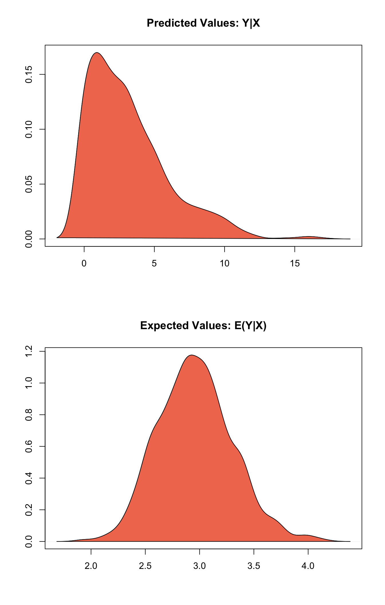
Graphs of Quantities of Interest for Zelig-negbin
Model
Let \(Y_i\) be the number of independent events that occur during a fixed time period. This variable can take any non-negative integer value.
- The negative binomial distribution is derived by letting the mean of the Poisson distribution vary according to a fixed parameter \(\zeta\) given by the Gamma distribution. The stochastic component is given by
\[ \begin{aligned} Y_i \mid \zeta_i & \sim & \textrm{Poisson}(\zeta_i \mu_i),\\ \zeta_i & \sim & \frac{1}{\theta}\textrm{Gamma}(\theta). \end{aligned} \] The marginal distribution of \(Y_i\) is then the negative binomial with mean \(\mu_i\) and variance \(\mu_i + \mu_i^2/\theta\):
\[ \begin{aligned} Y_i & \sim & \textrm{NegBin}(\mu_i, \theta), \\ & = & \frac{\Gamma (\theta + y_i)}{y! \, \Gamma(\theta)} \frac{\mu_i^{y_i} \, \theta^{\theta}}{(\mu_i + \theta)^{\theta + y_i}}, \end{aligned} \] where \(\theta\) is the systematic parameter of the Gamma distribution modeling \(\zeta_i\).
- The systematic component is given by
\[ \mu_i = \exp(x_i \beta) \]
where \(x_i\) is the vector of \(k\) explanatory variables and \(\beta\) is the vector of coefficients.
Quantities of Interest
- The expected values (qi$ev) are simulations of the mean of the stochastic component. Thus,
\[ E(Y) = \mu_i = \exp(x_i \beta), \]
given simulations of \(\beta\).
The predicted value (qi$pr) drawn from the distribution defined by the set of parameters \((\mu_i, \theta)\).
The first difference (qi$fd) is
\[ \textrm{FD} \; = \; E(Y | x_1) - E(Y \mid x) \]
- In conditional prediction models, the average expected treatment effect (att.ev) for the treatment group is
\[ \frac{1}{\sum_{i=1}^n t_i}\sum_{i:t_i=1}^n \left\{ Y_i(t_i=1) - E[Y_i(t_i=0)] \right\}, \]
where \(t_i\) is a binary explanatory variable defining the treatment (\(t_i=1\)) and control (\(t_i=0\)) groups. Variation in the simulations are due to uncertainty in simulating \(E[Y_i(t_i=0)]\), the counterfactual expected value of \(Y_i\) for observations in the treatment group, under the assumption that everything stays the same except that the treatment indicator is switched to \(t_i=0\).
- In conditional prediction models, the average predicted treatment effect (att.pr) for the treatment group is
\[ \frac{1}{\sum_{i=1}^n t_i}\sum_{i:t_i=1}^n \left\{ Y_i(t_i=1) - \widehat{Y_i(t_i=0)} \right\}, \]
where \(t_i\) is a binary explanatory variable defining the treatment (\(t_i=1\)) and control (\(t_i=0\)) groups. Variation in the simulations are due to uncertainty in simulating \(\widehat{Y_i(t_i=0)}\), the counterfactual predicted value of \(Y_i\) for observations in the treatment group, under the assumption that everything stays the same except that the treatment indicator is switched to \(t_i=0\).
Output Values
The Zelig object stores fields containing everything needed to rerun the Zelig output, and all the results and simulations as they are generated. In addition to the summary commands demonstrated above, some simply utility functions (known as getters) provide easy access to the raw fields most commonly of use for further investigation.
In the example above z.out$get_coef() returns the estimated coefficients, z.out$get_vcov() returns the estimated covariance matrix, and z.out$get_predict() provides predicted values for all observations in the dataset from the analysis.
See also
The negative binomial model is part of the MASS package by William N. Venable and Brian D. Ripley . Advanced users may wish to refer to help(glm.nb).
Venables WN and Ripley BD (2002). Modern Applied Statistics with S, Fourth edition. Springer, New York. ISBN 0-387-95457-0, <URL: http://www.stats.ox.ac.uk/pub/MASS4>.