Normal Linear Regression

Built using Zelig version 5.1.4.90000

Normal Regression for Continuous Dependent Variables with normal.

The Normal regression model is a close variant of the more standard least squares regression model. Both models specify a continuous dependent variable as a linear function of a set of explanatory variables. The Normal model reports maximum likelihood (rather than least squares) estimates. The two models differ only in their estimate for the stochastic parameter $\sigma$.

Syntax

z.out <- zelig(Y ~ X1 + X2, model = "normal", weights = w,
               data = mydata)
x.out <- setx(z.out)
s.out <- sim(z.out, x = x.out)

Examples

Basic Example with First Differences

Attach sample data:

data(macro)

Estimate model:

z.out1 <- zelig(unem ~ gdp + capmob + trade, model = "normal",
                data = macro)

## How to cite this model in Zelig:
##   R Core Team. 2008.
##   normal: Normal Regression for Continuous Dependent Variables
##   in Christine Choirat, Christopher Gandrud, James Honaker, Kosuke Imai, Gary King, and Olivia Lau,
##   "Zelig: Everyone's Statistical Software," http://zeligproject.org/

Summarize of regression coefficients:

summary(z.out1)

## Model: 
## 
## Call:
## z5$zelig(formula = unem ~ gdp + capmob + trade, data = macro)
## 
## Deviance Residuals: 
##     Min       1Q   Median       3Q      Max  
## -5.3008  -2.0768  -0.3187   1.9789   7.7715  
## 
## Coefficients:
##              Estimate Std. Error t value Pr(>|t|)
## (Intercept)  6.181294   0.450572  13.719  < 2e-16
## gdp         -0.323601   0.062820  -5.151 4.36e-07
## capmob       1.421939   0.166443   8.543 4.22e-16
## trade        0.019854   0.005606   3.542 0.000452
## 
## (Dispersion parameter for gaussian family taken to be 7.54307)
## 
##     Null deviance: 3664.8  on 349  degrees of freedom
## Residual deviance: 2609.9  on 346  degrees of freedom
## AIC: 1706.5
## 
## Number of Fisher Scoring iterations: 2
## 
## Next step: Use 'setx' method

Set explanatory variables to their default (mean/mode) values, with high (80th percentile) and low (20th percentile) values for trade:

x.high <- setx(z.out1, trade = quantile(macro$trade, 0.8))
x.low <- setx(z.out1, trade = quantile(macro$trade, 0.2))

Generate first differences for the effect of high versus low trade on GDP:

s.out1 <- sim(z.out1, x = x.high, x1 = x.low)

summary(s.out1)

## 
##  sim x :
##  -----
## ev
##          mean        sd     50%     2.5%    97.5%
## [1,] 5.439167 0.1843065 5.44302 5.074196 5.781827
## pv
##          mean       sd     50%      2.5%    97.5%
## [1,] 5.463443 2.713865 5.41136 0.4059531 10.85049
## 
##  sim x1 :
##  -----
## ev
##          mean        sd      50%     2.5%    97.5%
## [1,] 4.609335 0.1795533 4.607639 4.261402 4.971085
## pv
##          mean       sd      50%      2.5%    97.5%
## [1,] 4.767879 2.662139 4.764892 -0.447583 10.00484
## fd
##            mean        sd        50%      2.5%      97.5%
## [1,] -0.8298316 0.2320023 -0.8266661 -1.299632 -0.3615469

A visual summary of quantities of interest:

plot(s.out1)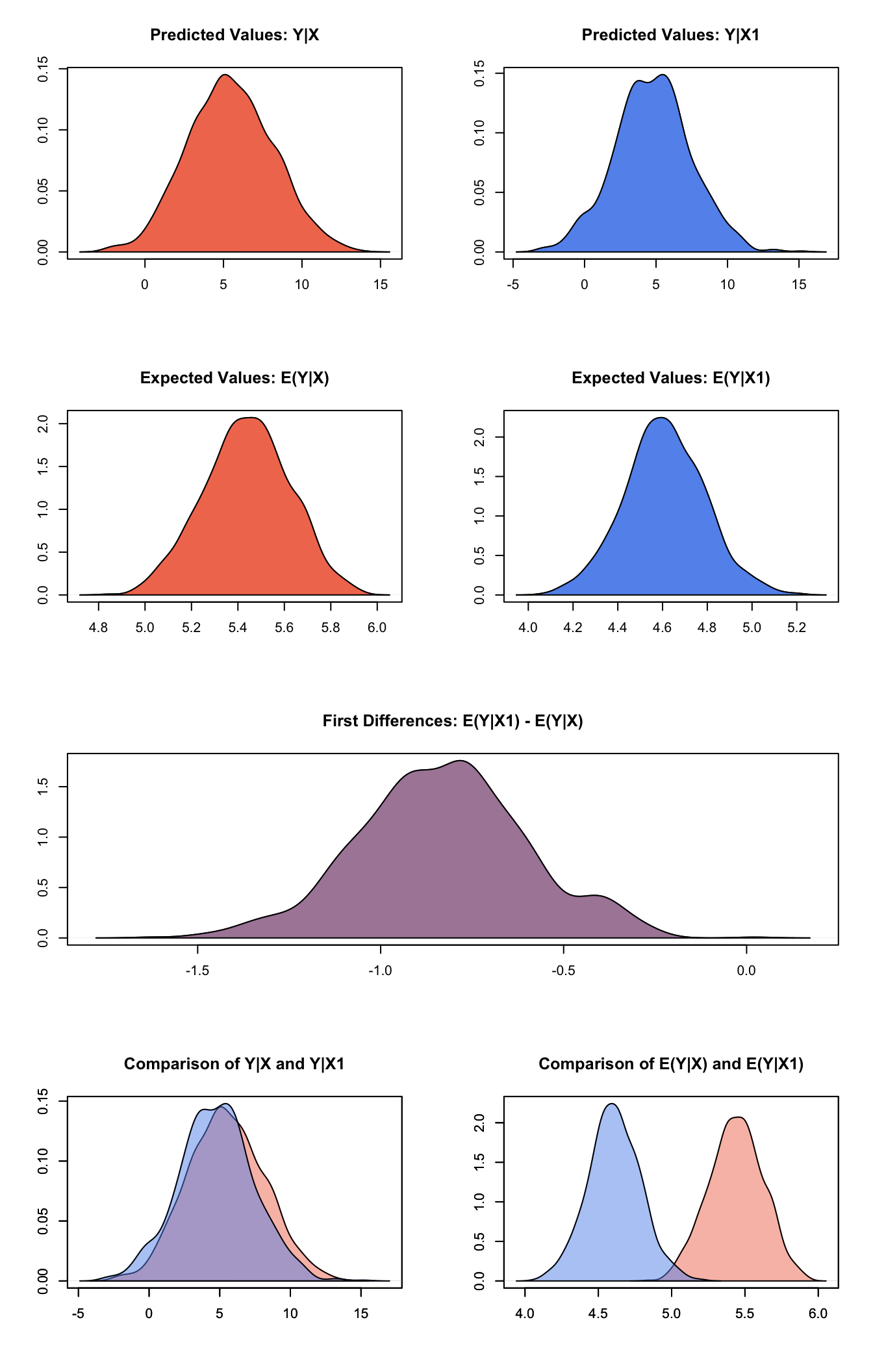

Graphs of Quantities of Interest for Zelig-normal

Model

Let $Y_i$ be the continuous dependent variable for observation $i$.

The stochastic component is described by a univariate normal model with a vector of means $\mu_i$ and scalar variance $\sigma^2$:

\[ Y_i \; \sim \; \textrm{Normal}(\mu_i, \sigma^2). \]

The systematic component is

\[ \mu_i \;= \; x_i \beta, \]

where $x_i$ is the vector of $k$ explanatory variables and $\beta$ is the vector of coefficients.

Quantities of Interest

The expected value (qi$ev) is the mean of simulations from the the stochastic component,

\[ E(Y) = \mu_i = x_i \beta, \]

given a draw of $\beta$ from its posterior.

The predicted value (qi$pr) is drawn from the distribution defined by the set of parameters $(\mu_i, \sigma)$.
The first difference (qi$fd) is:

\[ \textrm{FD}\; = \;E(Y \mid x_1) - E(Y \mid x) \]

In conditional prediction models, the average expected treatment effect (att.ev) for the treatment group is

\[ \frac{1}{\sum_{i=1}^n t_i}\sum_{i:t_i=1}^n \left\{ Y_i(t_i=1) - E[Y_i(t_i=0)] \right\}, \]

where $t_i$ is a binary explanatory variable defining the treatment ($t_i=1$) and control ($t_i=0$) groups. Variation in the simulations are due to uncertainty in simulating $E[Y_i(t_i=0)]$, the counterfactual expected value of $Y_i$ for observations in the treatment group, under the assumption that everything stays the same except that the treatment indicator is switched to $t_i=0$.

In conditional prediction models, the average predicted treatment effect (att.pr) for the treatment group is

\[ \frac{1}{\sum_{i=1}^n t_i}\sum_{i:t_i=1}^n \left\{ Y_i(t_i=1) - \widehat{Y_i(t_i=0)} \right\}, \]

where $t_i$ is a binary explanatory variable defining the treatment ($t_i=1$) and control ($t_i=0$) groups. Variation in the simulations are due to uncertainty in simulating $\widehat{Y_i(t_i=0)}$, the counterfactual predicted value of $Y_i$ for observations in the treatment group, under the assumption that everything stays the same except that the treatment indicator is switched to $t_i=0$.

Output Values

The Zelig object stores fields containing everything needed to rerun the Zelig output, and all the results and simulations as they are generated. In addition to the summary commands demonstrated above, some simply utility functions (known as getters) provide easy access to the raw fields most commonly of use for further investigation.

If the zelig() call output object is z.out, then coef(z.out) returns the estimated coefficients, vcov(z.out) returns the estimated covariance matrix, and predict(z.out) provides predicted values for all observations in the dataset from the analysis.

2017-10-29