Normal Survey Regression
2017-10-29
Built using Zelig version 5.1.4.90000
Normal Regression for Continuous Dependent Variables with Survey Weights with normal.survey.
The Normal regression model is a close variant of the more standard least squares regression model (see Normal Regress). Both models specify a continuous dependent variable as a linear function of a set of explanatory variables. The Normal model reports maximum likelihood (rather than least squares) estimates. The two models differ only in their estimate for the stochastic parameter \(\sigma\).
Examples
Example 1: User has Existing Sample Weights
Attach sample data and variable names:
data(api, package = "survey")In this example, we will estimate a model using the percentages of students who receive subsidized lunch (meals) and an indicator for whether schooling is year-round (yr.rnd) to predict California public schools’ academic performance index scores (api00). Sampling weights are stored in a variable called pw.
z.out1 <- zelig(api00 ~ meals + yr.rnd, model = "normal.survey",
                weights = ~pw, data = apistrat)
## Warning: Not all features are available in Zelig Survey.
## Consider using surveyglm and setx directly.
## For details see: <http://docs.zeligproject.org/articles/to_zelig.html>.## How to cite this model in Zelig:
## Nicholas Carnes. 2017.
## normal-survey: Normal Regression for Continuous Dependent Variables with Survey Weights
## in Christine Choirat, Christopher Gandrud, James Honaker, Kosuke Imai, Gary King, and Olivia Lau,
## "Zelig: Everyone's Statistical Software," http://zeligproject.org/summary(z.out1)## Model:
##
## Call:
## z5$zelig(formula = api00 ~ meals + yr.rnd, data = apistrat, weights = ~pw)
##
## Survey design:
## survey::svydesign(data = data, ids = ids, probs = probs, strata = strata,
## fpc = fpc, nest = nest, check.strata = check.strata, weights = localWeights)
##
## Coefficients:
## Estimate Std. Error t value Pr(>|t|)
## (Intercept) 846.0409 8.9836 94.176 <2e-16
## meals -3.4882 0.1678 -20.783 <2e-16
## yr.rndYes -15.4566 15.6413 -0.988 0.324
##
## (Dispersion parameter for gaussian family taken to be 155138.3)
##
## Number of Fisher Scoring iterations: 2
##
## Next step: Use 'setx' methodSet explanatory variables to their default (mean/mode) values, and set a high (80th percentile) and low (20th percentile) value for “meals,” the percentage of students who receive subsidized meals:
x.low <- setx(z.out1, meals = quantile(apistrat$meals, 0.2))
x.high <- setx(z.out1, meals = quantile(apistrat$meals, 0.8))
Generate first differences for the effect of high versus low “meals” on academic performance:
s.out1 <- sim(z.out1, x = x.high, x1 = x.low)
summary(s.out1)
##
## sim x :
## -----
## ev
## mean sd 50% 2.5% 97.5%
## [1,] 587.3657 7.32722 587.2933 572.4778 602.4199
## pv
## mean sd 50% 2.5% 97.5%
## [1,] 606.9886 376.4908 611.1407 -123.9886 1307.963
##
## sim x1 :
## -----
## ev
## mean sd 50% 2.5% 97.5%
## [1,] 783.0764 6.718347 783.2417 770.1292 796.5756
## pv
## mean sd 50% 2.5% 97.5%
## [1,] 786.6935 390.9711 777.5449 48.42074 1567.279
## fd
## mean sd 50% 2.5% 97.5%
## [1,] 195.7107 9.248029 195.8242 178.0784 213.7883Generate a second set of fitted values and a plot:
plot(s.out1)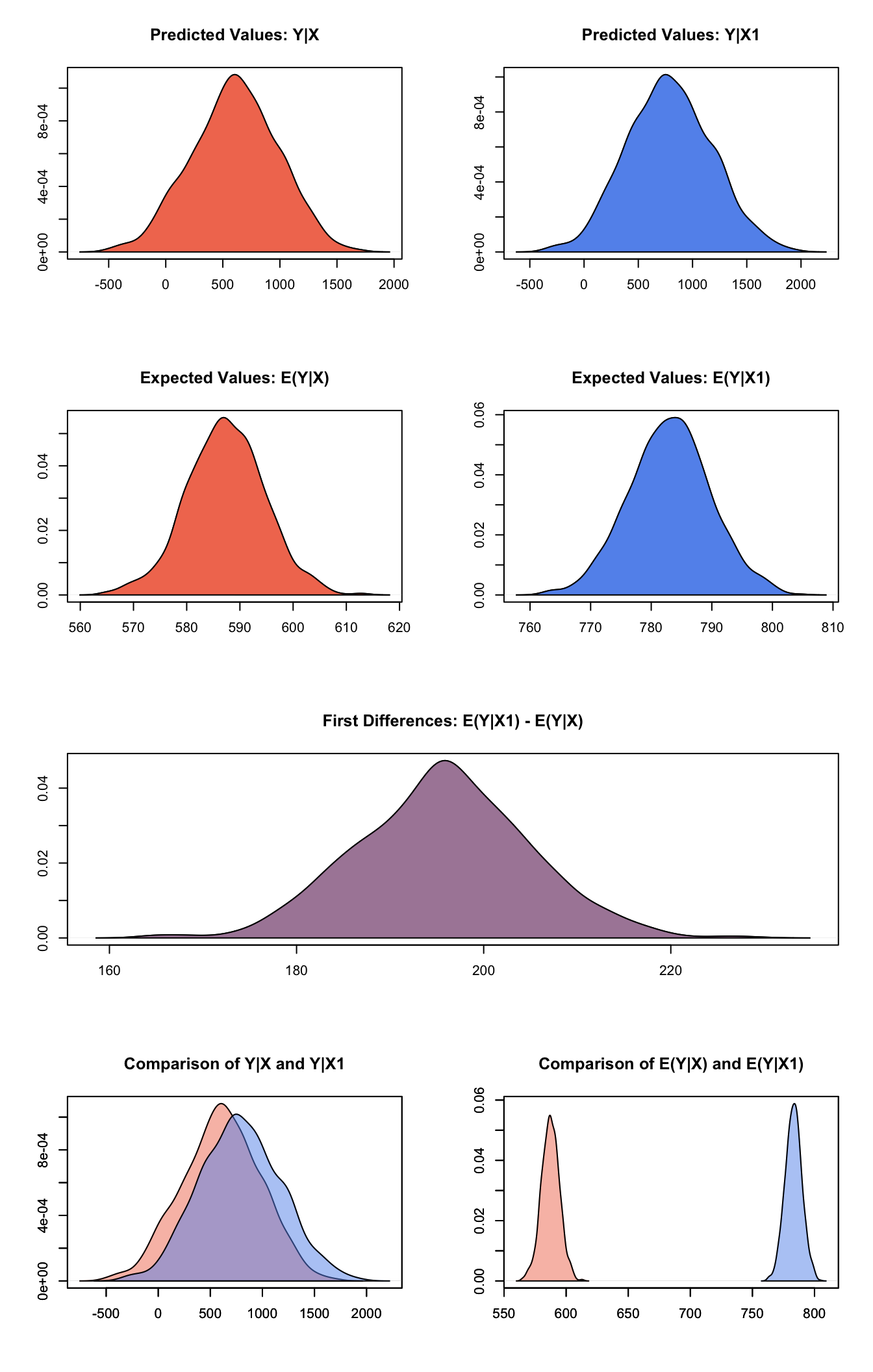
Graphs of Quantities of Interest for Normal Survey Model
Example 2: User has Details about Complex Survey Design (but not sample weights)
Suppose that the survey house that provided the dataset excluded probability weights but made other details about the survey design available. We can still estimate a model without probability weights that takes instead variables that identify each the stratum and/or cluster from which each observation was selected and the size of the finite sample from which each observation was selected.
z.out2 <- zelig(api00 ~ meals + yr.rnd, model = "normal.survey",
                strata = ~stype, fpc = ~fpc, data = apistrat)
## Warning: Not all features are available in Zelig Survey.
## Consider using surveyglm and setx directly.
## For details see: <http://docs.zeligproject.org/articles/to_zelig.html>.## How to cite this model in Zelig:
## Nicholas Carnes. 2017.
## normal-survey: Normal Regression for Continuous Dependent Variables with Survey Weights
## in Christine Choirat, Christopher Gandrud, James Honaker, Kosuke Imai, Gary King, and Olivia Lau,
## "Zelig: Everyone's Statistical Software," http://zeligproject.org/summary(z.out2)## Model:
##
## Call:
## z5$zelig(formula = api00 ~ meals + yr.rnd, data = apistrat, strata = ~stype,
## fpc = ~fpc)
##
## Survey design:
## survey::svydesign(data = data, ids = ids, probs = probs, strata = strata,
## fpc = fpc, nest = nest, check.strata = check.strata, weights = localWeights)
##
## Coefficients:
## Estimate Std. Error t value Pr(>|t|)
## (Intercept) 825.1058 8.3552 98.753 <2e-16
## meals -3.3581 0.1644 -20.430 <2e-16
## yr.rndYes -6.3855 15.1624 -0.421 0.674
##
## (Dispersion parameter for gaussian family taken to be 5225.087)
##
## Number of Fisher Scoring iterations: 2
##
## Next step: Use 'setx' methodNote that these results are identical to the results obtained when pre-existing sampling weights were used. When sampling weights are omitted, Zelig estimates them automatically for “normal.survey” models based on the user-defined description of sampling designs. If no description is present, the default assumption is equal probability sampling.
The methods setx() and sim() can then be run on z.out2 in the same fashion described above.
Example 3: User has Replicate Weights
Load data for a model using the number of out-of-hospital cardiac arrests to predict the number of patients who arrive alive in hospitals:
data(scd, package = "survey")Create four Balanced Repeated Replicate (BRR) weights:
BRRrep <- 2*cbind(c(1,0,1,0,1,0), c(1,0,0,1,0,1),
                c(0,1,1,0,0,1), c(0,1,0,1,1,0))
Estimate the model using Zelig:
z.out3 <- zelig(formula=alive ~ arrests , model = "normal.survey",
                repweights = BRRrep, type = "BRR",
                data = scd, na.action = NULL)
## Warning: Not all features are available in Zelig Survey.
## Consider using surveyglm and setx directly.
## For details see: <http://docs.zeligproject.org/articles/to_zelig.html>.## Warning in svrepdesign.default(data = data, repweights = repweights, type =
## type, : No sampling weights provided: equal probability assumed## How to cite this model in Zelig:
## Nicholas Carnes. 2017.
## normal-survey: Normal Regression for Continuous Dependent Variables with Survey Weights
## in Christine Choirat, Christopher Gandrud, James Honaker, Kosuke Imai, Gary King, and Olivia Lau,
## "Zelig: Everyone's Statistical Software," http://zeligproject.org/summary(z.out3)## Model:
##
## Call:
## z5$zelig(formula = alive ~ arrests, data = scd, repweights = BRRrep,
## type = "BRR", na.action = NULL)
##
## Survey design:
## svrepdesign.default(data = data, repweights = repweights, type = type,
## weights = localWeights, combined.weights = combined.weights,
## rho = rho, bootstrap.average = bootstrap.average, scale = scale,
## rscales = rscales, fpctype = fpctype, fpc = fpc)
##
## Coefficients:
## Estimate Std. Error t value Pr(>|t|)
## (Intercept) 16.777828 3.949296 4.248 0.05119
## arrests 0.097920 0.006064 16.149 0.00381
##
## (Dispersion parameter for gaussian family taken to be 23.65681)
##
## Number of Fisher Scoring iterations: 2
##
## Next step: Use 'setx' methodSet the explanatory variable at its minimum and maximum
Generate first differences for the effect of the minimum versus the maximum number of cardiac arrests on the number of people who arrive alive:
s.out3 <- sim(z.out3, x=x.max, x1=x.min)
summary(s.out3)
##
## sim x :
## -----
## ev
## mean sd 50% 2.5% 97.5%
## [1,] 24.47312 3.603297 24.56658 17.75726 31.51732
## pv
## mean sd 50% 2.5% 97.5%
## [1,] 24.41233 12.22076 24.53819 2.84381 45.37047
##
## sim x1 :
## -----
## ev
## mean sd 50% 2.5% 97.5%
## [1,] 18.97948 3.876408 19.06842 11.69499 26.37252
## pv
## mean sd 50% 2.5% 97.5%
## [1,] 19.47485 12.3683 18.89057 -0.7115458 40.6895
## fd
## mean sd 50% 2.5% 97.5%
## [1,] -5.493631 0.3337031 -5.489195 -6.142893 -4.83746Generate a second set of fitted values and a plot:
plot(s.out3)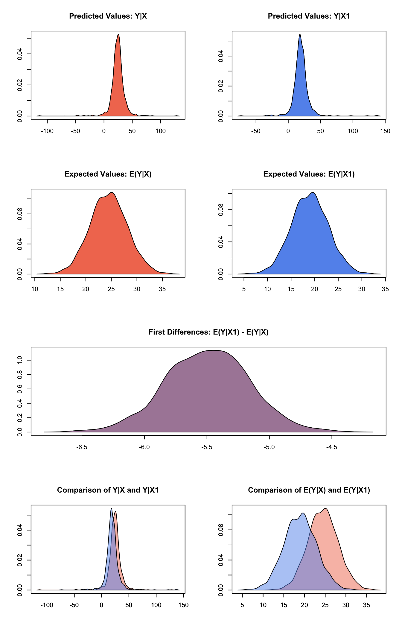
Graphs of Quantities of Interest for Normal Survey Model
The user should also refer to the normal model demo, since normal.survey models can take many of the same options as normal models.
Model
Let \(Y_i\) be the continuous dependent variable for observation \(i\).
- The stochastic component is described by a univariate normal model with a vector of means \(\mu_i\) and scalar variance \(\sigma^2\):
\[ Y_i \; \sim \; \textrm{Normal}(\mu_i, \sigma^2). \]
- The systematic component is
\[ \mu_i \;= \; x_i \beta, \]
where \(x_i\) is the vector of \(k\) explanatory variables and \(\beta\) is the vector of coefficients.
Quantities of Interest
- The expected value (qi$ev) is the mean of simulations from the the stochastic component,
\[ E(Y) = \mu_i = x_i \beta, \]
given a draw of \(\beta\) from its posterior.
The predicted value (qi$pr) is drawn from the distribution defined by the set of parameters \((\mu_i, \sigma)\).
The first difference (qi$fd) is:
\[ \textrm{FD}\; = \;E(Y \mid x_1) - E(Y \mid x) \]
- In conditional prediction models, the average expected treatment effect (att.ev) for the treatment group is
\[ \frac{1}{\sum_{i=1}^n t_i}\sum_{i:t_i=1}^n \left\{ Y_i(t_i=1) - E[Y_i(t_i=0)] \right\}, \]
where \(t_i\) is a binary explanatory variable defining the treatment (\(t_i=1\)) and control (\(t_i=0\)) groups. Variation in the simulations are due to uncertainty in simulating \(E[Y_i(t_i=0)]\), the counterfactual expected value of \(Y_i\) for observations in the treatment group, under the assumption that everything stays the same except that the treatment indicator is switched to \(t_i=0\).
- In conditional prediction models, the average predicted treatment effect (att.pr) for the treatment group is
\[ \frac{1}{\sum_{i=1}^n t_i}\sum_{i:t_i=1}^n \left\{ Y_i(t_i=1) - \widehat{Y_i(t_i=0)} \right\}, \]
where \(t_i\) is a binary explanatory variable defining the treatment (\(t_i=1\)) and control (\(t_i=0\)) groups. Variation in the simulations are due to uncertainty in simulating \(\widehat{Y_i(t_i=0)}\), the counterfactual predicted value of \(Y_i\) for observations in the treatment group, under the assumption that everything stays the same except that the treatment indicator is switched to \(t_i=0\).
Output Values
The Zelig object stores fields containing everything needed to rerun the Zelig output, and all the results and simulations as they are generated. In addition to the summary commands demonstrated above, some simply utility functions (known as getters) provide easy access to the raw fields most commonly of use for further investigation.
In the example above z.out$get_coef() returns the estimated coefficients, z.out$get_vcov() returns the estimated covariance matrix, and z.out$get_predict() provides predicted values for all observations in the dataset from the analysis.
See also
The normalsurvey model is part of the survey package by Thomas Lumley, which in turn depends heavily on glm package. Advanced users may wish to refer to help(svyglm) and help(family).
Lumley T (2016). “survey: analysis of complex survey samples.” R package version 3.32.
Lumley T (2004). “Analysis of Complex Survey Samples.” Journal of Statistical Software, 9 (1), pp. 1-19. R package verson 2.2.