Poisson

Built using Zelig version 5.1.4.90000

Poisson Regression for Event Count Dependent Variables with poisson.

Use the Poisson regression model if the observations of your dependent variable represents the number of independent events that occur during a fixed period of time (see the negative binomial model, , for over-dispersed event counts.) For a Bayesian implementation of this model, see .

Syntax

z.out <- zelig(Y ~ X1 + X2, model = "poisson", weights = w, data = mydata)
x.out <- setx(z.out)
s.out <- sim(z.out, x = x.out)

Example

Load sample data:

data(sanction)

Estimate Poisson model:

z.out <- zelig(num ~ target + coop, model = "poisson", data = sanction)

## How to cite this model in Zelig:
##   R Core Team. 2007.
##   poisson: Poisson Regression for Event Count Dependent Variables
##   in Christine Choirat, Christopher Gandrud, James Honaker, Kosuke Imai, Gary King, and Olivia Lau,
##   "Zelig: Everyone's Statistical Software," http://zeligproject.org/

summary(z.out)

## Model: 
## 
## Call:
## z5$zelig(formula = num ~ target + coop, data = sanction)
## 
## Deviance Residuals: 
##     Min       1Q   Median       3Q      Max  
## -7.2127  -1.1831  -0.2080  -0.1856  17.6514  
## 
## Coefficients:
##             Estimate Std. Error z value Pr(>|z|)
## (Intercept) -0.96772    0.17545  -5.516 3.48e-08
## target      -0.02102    0.05823  -0.361    0.718
## coop         1.21082    0.04662  25.970  < 2e-16
## 
## (Dispersion parameter for poisson family taken to be 1)
## 
##     Null deviance: 1583.77  on 77  degrees of freedom
## Residual deviance:  720.84  on 75  degrees of freedom
## AIC: 944.35
## 
## Number of Fisher Scoring iterations: 6
## 
## Next step: Use 'setx' method

Set values for the explanatory variables to their default mean values, while changing the $coop$ variable across its range:

x.low <- setx(z.out, coop = 1)
x.high <- setx1(z.out, coop = 4)

Simulate fitted values:

s.out <- sim(z.out, x = x.low, x1=x.high)
summary(s.out)

## 
##  sim x :
##  -----
## ev
##         mean        sd      50%      2.5%    97.5%
## [1,] 1.22071 0.1225477 1.214888 0.9981235 1.474667
## pv
##       mean       sd 50% 2.5% 97.5%
## [1,] 1.239 1.089526   1    0     4
## 
##  sim x1 :
##  -----
## ev
##         mean      sd      50%     2.5%    97.5%
## [1,] 46.1529 2.87779 46.10616 40.50223 52.03349
## pv
##        mean       sd 50%   2.5% 97.5%
## [1,] 45.734 7.150831  46 32.975    60
## fd
##          mean       sd    50%     2.5%    97.5%
## [1,] 44.93219 2.922241 44.872 39.28703 50.96481

plot(s.out)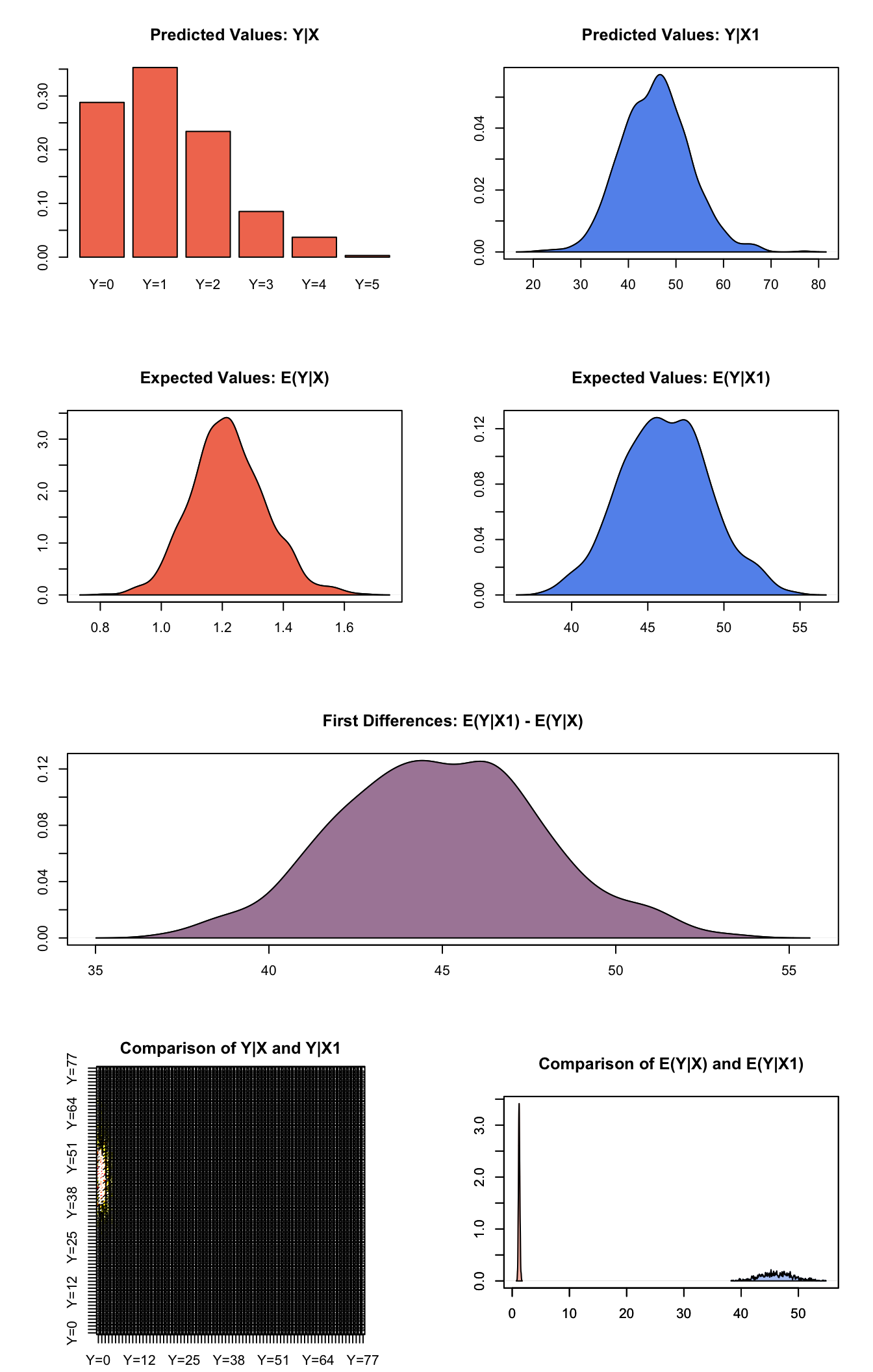

Graphs of Quantities of Interest for Zelig-poisson

Model

Let $Y_i$ be the number of independent events that occur during a fixed time period. This variable can take any non-negative integer.

The Poisson distribution has stochastic component

\[ Y_i \; \sim \; \textrm{Poisson}(\lambda_i), \]

where $\lambda_i$ is the mean and variance parameter.

The systematic component is

\[ \lambda_i \; = \; \exp(x_i \beta), \]

where $x_i$ is the vector of explanatory variables, and $\beta$ is the vector of coefficients.

Quantities of Interest

The expected value (qi$ev) is the mean of simulations from the stochastic component,

\[ E(Y) = \lambda_i = \exp(x_i \beta), \]

given draws of $\beta$ from its sampling distribution.

The predicted value (qi$pr) is a random draw from the poisson distribution defined by mean $\lambda_i$.
The first difference in the expected values (qi$fd) is given by:

\[ \textrm{FD} \; = \; E(Y | x_1) - E(Y \mid x) \]

In conditional prediction models, the average expected treatment effect (att.ev) for the treatment group is

\[ \frac{1}{\sum_{i=1}^n t_i}\sum_{i:t_i=1}^n \left\{ Y_i(t_i=1) - E[Y_i(t_i=0)] \right\}, \]

where $t_i$ is a binary explanatory variable defining the treatment ($t_i=1$) and control ($t_i=0$) groups. Variation in the simulations are due to uncertainty in simulating $E[Y_i(t_i=0)]$, the counterfactual expected value of $Y_i$ for observations in the treatment group, under the assumption that everything stays the same except that the treatment indicator is switched to $t_i=0$.

In conditional prediction models, the average predicted treatment effect (att.pr) for the treatment group is

\[ \frac{1}{\sum_{i=1}^n t_i}\sum_{i:t_i=1}^n \left\{ Y_i(t_i=1) - \widehat{Y_i(t_i=0)} \right\}, \]

where $t_i$ is a binary explanatory variable defining the treatment ($t_i=1$) and control ($t_i=0$) groups. Variation in the simulations are due to uncertainty in simulating $\widehat{Y_i(t_i=0)}$, the counterfactual predicted value of $Y_i$ for observations in the treatment group, under the assumption that everything stays the same except that the treatment indicator is switched to $t_i=0$.

Output Values

The Zelig object stores fields containing everything needed to rerun the Zelig output, and all the results and simulations as they are generated. In addition to the summary commands demonstrated above, some simply utility functions (known as getters) provide easy access to the raw fields most commonly of use for further investigation.

In the example above z.out$get_coef() returns the estimated coefficients, z.out$get_vcov() returns the estimated covariance matrix, and z.out$get_predict() provides predicted values for all observations in the dataset from the analysis.

2017-10-29

Syntax

Example

Model

Quantities of Interest

Output Values

See also

Contents