Poisson Survey Regression

Built using Zelig version 5.1.4.90000

Poisson Regression for Event Count Dependent Variables with Survey Weights with poisson.survey.

Use the Poisson regression model if the observations of your dependent variable represents the number of independent events that occur during a fixed period of time (see the negative binomial model for over-dispersed event counts.) For a Bayesian implementation of this model, see Zelig Poisson Bayes.

Syntax

z.out <- zelig(Y ~ X1 + X2, model = "poisson.survey",
               weights = w, data = mydata)
x.out <- setx(z.out)
s.out <- sim(z.out, x = x.out)

Example

Example 1: User has Existing Sample Weights

Attach sample data:

data(api, package="survey")

In this example, we will estimate a model using each school’s academic performance in 2000 and an indicator for year-round schools to predict the number of students who enrolled in each California school.

z.out1 <- zelig(enroll ~ api99 + yr.rnd ,
                model = "poisson.survey", data = apistrat)

## Warning: Not all features are available in Zelig Survey.
## Consider using surveyglm and setx directly.
## For details see: <http://docs.zeligproject.org/articles/to_zelig.html>.

## How to cite this model in Zelig:
##   Nicholas Carnes. 2017.
##   poisson-survey: Poisson Regression with Survey Weights
##   in Christine Choirat, Christopher Gandrud, James Honaker, Kosuke Imai, Gary King, and Olivia Lau,
##   "Zelig: Everyone's Statistical Software," http://zeligproject.org/

summary(z.out1)

## Model: 
## 
## Call:
## z5$zelig(formula = enroll ~ api99 + yr.rnd, data = apistrat)
## 
## Survey design:
## survey::svydesign(data = data, ids = ids, probs = probs, strata = strata, 
##     fpc = fpc, nest = nest, check.strata = check.strata, weights = localWeights)
## 
## Coefficients:
##               Estimate Std. Error t value Pr(>|t|)
## (Intercept)  7.1282917  0.2645220  26.948   <2e-16
## api99       -0.0008395  0.0004091  -2.052   0.0415
## yr.rndYes    0.0556202  0.1730477   0.321   0.7482
## 
## (Dispersion parameter for poisson family taken to be 391.138)
## 
## Number of Fisher Scoring iterations: 5
## 
## Next step: Use 'setx' method

Set explanatory variables to their default (mean/mode) values, and set a high (80th percentile) and low (20th percentile) value for the measure of academic performance, “api00”:

x.low <- setx(z.out1, api99= quantile(apistrat$api99, 0.2))
x.high <- setx(z.out1, api99= quantile(apistrat$api99, 0.8))

Generate first differences for the effect of high versus low “meals” on the probability that a school will hold classes year round:

s.out1 <- sim(z.out1, x=x.low, x1=x.high)
summary(s.out1)

## 
##  sim x :
##  -----
## ev
##          mean       sd      50%     2.5%   97.5%
## [1,] 817.1636 61.73815 815.3758 704.7528 941.267
## pv
##        mean       sd 50%   2.5% 97.5%
## [1,] 818.18 67.05647 817 688.95 953.1
## 
##  sim x1 :
##  -----
## ev
##          mean       sd      50%     2.5%    97.5%
## [1,] 671.6269 47.28784 670.2435 583.5333 769.5095
## pv
##         mean       sd   50%    2.5%   97.5%
## [1,] 671.552 53.03488 670.5 566.975 773.025
## fd
##           mean       sd       50%      2.5%     97.5%
## [1,] -145.5367 72.31272 -144.6802 -288.4826 -9.957065

Generate a second set of fitted values and a plot:

plot(s.out1)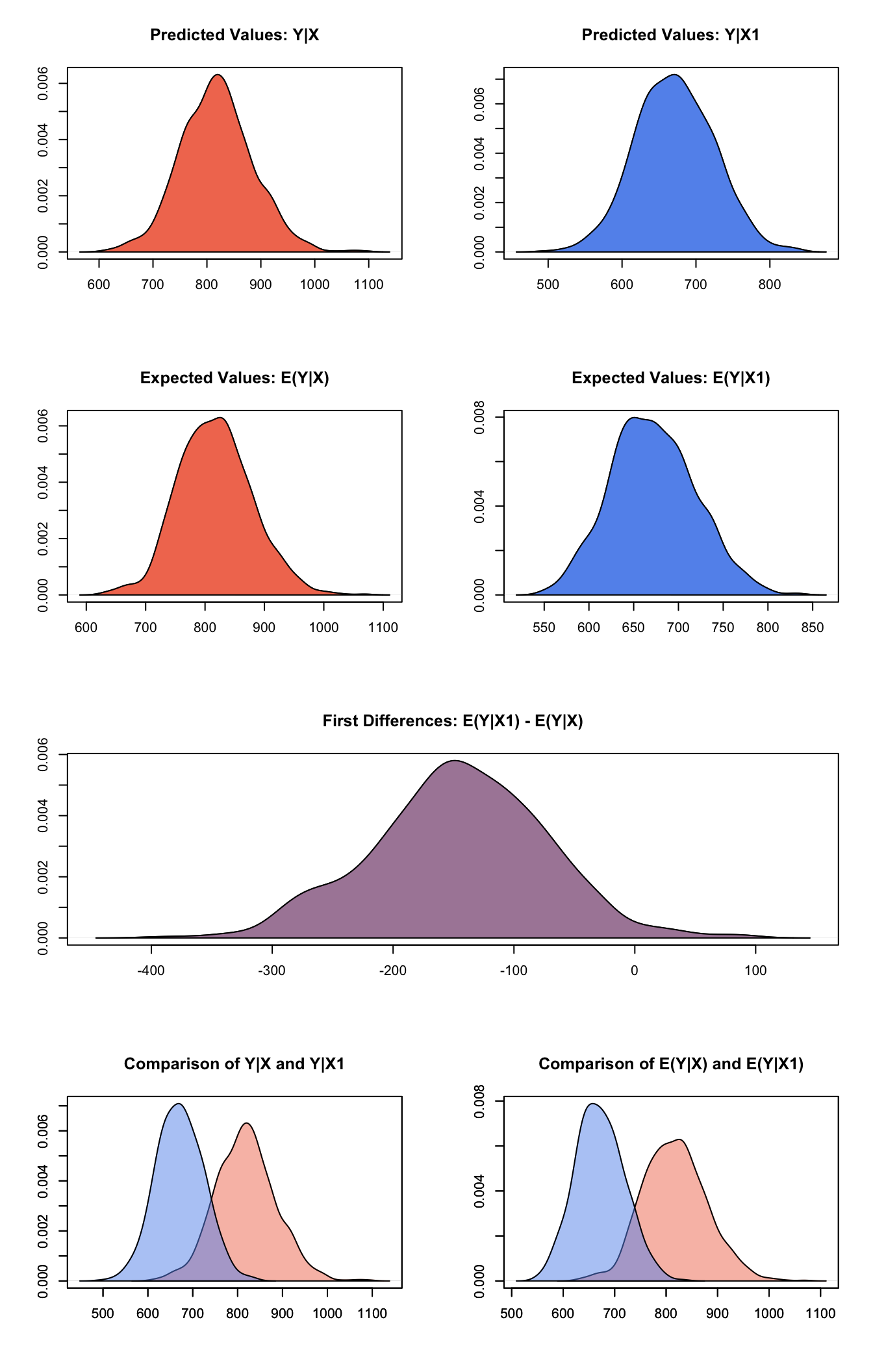

Graphs of Quantities of Interest for Poisson Survey Model

Example 2: User has Details about Complex Survey Design (but not sample weights)

Suppose that the survey house that provided the dataset excluded probability weights but made other details about the survey design available. We can still estimate a model without probability weights that takes instead variables that identify each the stratum and/or cluster from which each observation was selected and the size of the finite sample from which each observation was selected.

z.out2 <- zelig(enroll ~ api99 + yr.rnd ,
                model = "poisson.survey", data = apistrat,
                strata = ~stype, fpc = ~fpc)

## Warning: Not all features are available in Zelig Survey.
## Consider using surveyglm and setx directly.
## For details see: <http://docs.zeligproject.org/articles/to_zelig.html>.

## How to cite this model in Zelig:
##   Nicholas Carnes. 2017.
##   poisson-survey: Poisson Regression with Survey Weights
##   in Christine Choirat, Christopher Gandrud, James Honaker, Kosuke Imai, Gary King, and Olivia Lau,
##   "Zelig: Everyone's Statistical Software," http://zeligproject.org/

summary(z.out2)

## Model: 
## 
## Call:
## z5$zelig(formula = enroll ~ api99 + yr.rnd, data = apistrat, 
##     strata = ~stype, fpc = ~fpc)
## 
## Survey design:
## survey::svydesign(data = data, ids = ids, probs = probs, strata = strata, 
##     fpc = fpc, nest = nest, check.strata = check.strata, weights = localWeights)
## 
## Coefficients:
##               Estimate Std. Error t value Pr(>|t|)
## (Intercept)  6.9287587  0.2177819  31.815  < 2e-16
## api99       -0.0008984  0.0003316  -2.709  0.00734
## yr.rndYes    0.1207127  0.1097426   1.100  0.27270
## 
## (Dispersion parameter for poisson family taken to be 314.0072)
## 
## Number of Fisher Scoring iterations: 5
## 
## Next step: Use 'setx' method

The coefficient estimates from this model are identical to point estimates in the previous example, but the standard errors are smaller. When sampling weights are omitted, Zelig estimates them automatically for “normal.survey” models based on the user-defined description of sampling designs. In addition, when user-defined descriptions of the sampling design are entered as inputs, variance estimates are better and standard errors are consequently smaller.

The methods setx() and sim() can then be run on z.out2 in the same fashion described in Example 1.

Example 3: User has Replicate Weights

Load data for a model using the number of out-of-hospital cardiac arrests to predict the number of patients who arrive alive in hospitals.

data(scd, package="survey")

For the purpose of illustration, create four Balanced Repeated Replicate (BRR) weights:

BRRrep<-2*cbind(c(1,0,1,0,1,0), c(1,0,0,1,0,1), c(0,1,1,0,0,1), c(0,1,0,1,1,0))

Estimate the model using Zelig:

z.out3 <- zelig(alive ~ arrests , model = "poisson.survey",
                repweights = BRRrep, type = "BRR", data = scd)

## Warning: Not all features are available in Zelig Survey.
## Consider using surveyglm and setx directly.
## For details see: <http://docs.zeligproject.org/articles/to_zelig.html>.

## Warning in svrepdesign.default(data = data, repweights = repweights, type =
## type, : No sampling weights provided: equal probability assumed

## How to cite this model in Zelig:
##   Nicholas Carnes. 2017.
##   poisson-survey: Poisson Regression with Survey Weights
##   in Christine Choirat, Christopher Gandrud, James Honaker, Kosuke Imai, Gary King, and Olivia Lau,
##   "Zelig: Everyone's Statistical Software," http://zeligproject.org/

summary(z.out3)

## Model: 
## 
## Call:
## z5$zelig(formula = alive ~ arrests, data = scd, repweights = BRRrep, 
##     type = "BRR")
## 
## Survey design:
## svrepdesign.default(data = data, repweights = repweights, type = type, 
##     weights = localWeights, combined.weights = combined.weights, 
##     rho = rho, bootstrap.average = bootstrap.average, scale = scale, 
##     rscales = rscales, fpctype = fpctype, fpc = fpc)
## 
## Coefficients:
##              Estimate Std. Error t value Pr(>|t|)
## (Intercept) 3.1552572  0.1426950  22.112  0.00204
## arrests     0.0019342  0.0002659   7.273  0.01838
## 
## (Dispersion parameter for poisson family taken to be 1.083471)
## 
## Number of Fisher Scoring iterations: 4
## 
## Next step: Use 'setx' method

Set the explanatory variables at their means and set arrests at its 20th and 80th quartiles

x.low <- setx(z.out3, arrests = quantile(scd$arrests, .2))
x.high <- setx(z.out3, arrests = quantile(scd$arrests,.8))

Generate first differences for the effect of the minimum versus the maximum number of individuals who arrive alive on the probability that a hospital will be sued:

s.out3 <- sim(z.out3, x=x.high, x1=x.low)
summary(s.out3)

## 
##  sim x :
##  -----
## ev
##          mean       sd      50%     2.5%    97.5%
## [1,] 65.25006 4.440585 65.11013 56.82662 74.35446
## pv
##        mean       sd 50% 2.5%  97.5%
## [1,] 65.254 9.006809  65   49 84.025
## 
##  sim x1 :
##  -----
## ev
##          mean       sd      50%     2.5%    97.5%
## [1,] 29.79284 3.519312 29.62834 23.44793 36.86325
## pv
##        mean       sd 50% 2.5% 97.5%
## [1,] 29.604 6.312768  29   18    43
## fd
##           mean       sd       50%      2.5%     97.5%
## [1,] -35.45722 4.405681 -35.40398 -44.63728 -27.07315

Generate a second set of fitted values and a plot:

plot(s.out3)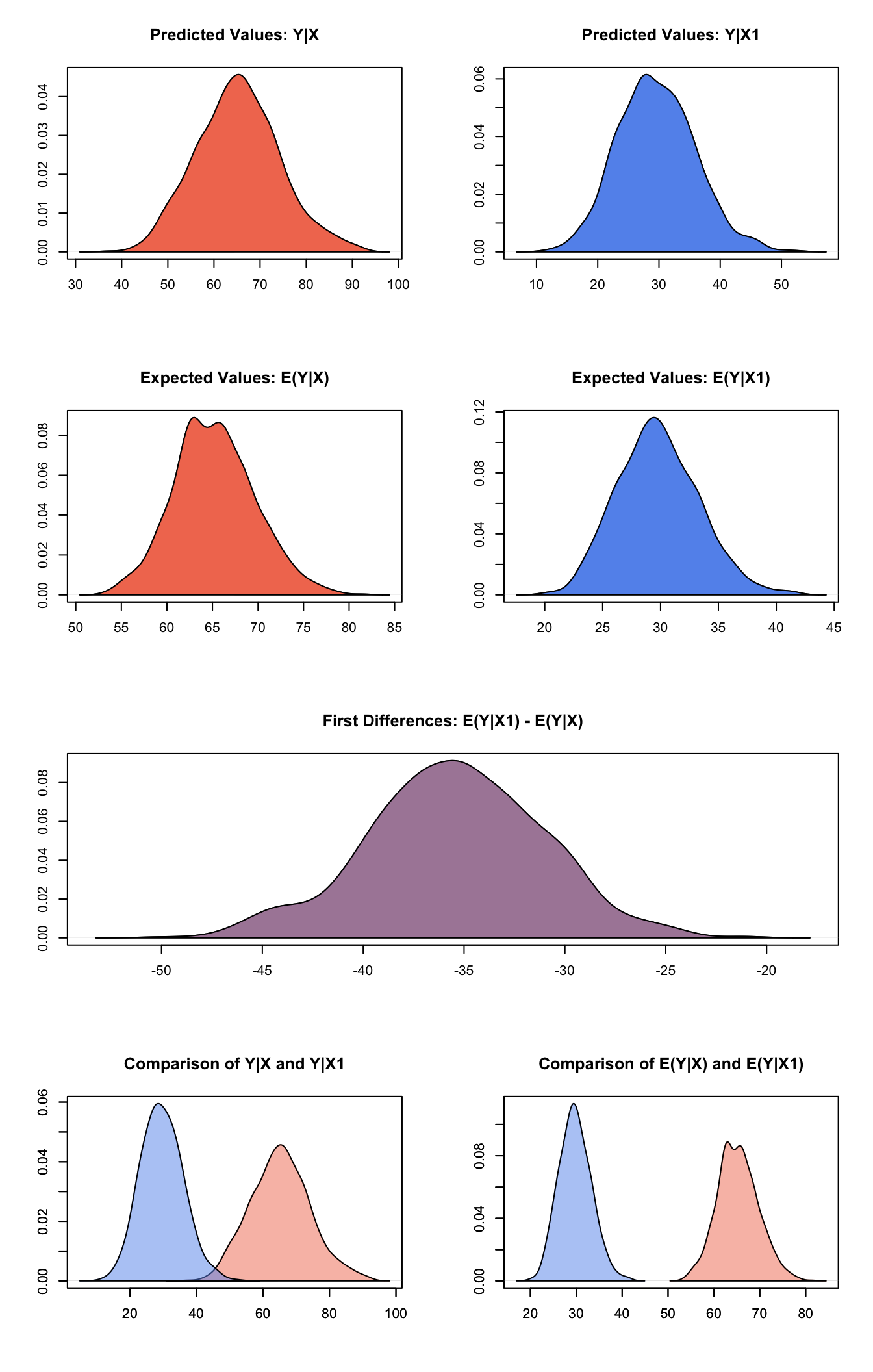

Graphs of Quantities of Interest for Poisson Survey Model

The user should also refer to the poisson model demo, since poisson.survey models can take many of the same options as poisson models.

Model

Let $Y_i$ be the number of independent events that occur during a fixed time period. This variable can take any non-negative integer.

The Poisson distribution has stochastic component

\[ Y_i \; \sim \; \textrm{Poisson}(\lambda_i), \]

where $\lambda_i$ is the mean and variance parameter.

The systematic component is

\[ \lambda_i \; = \; \exp(x_i \beta), \]

where $x_i$ is the vector of explanatory variables, and $\beta$ is the vector of coefficients.

Quantities of Interest

The expected value (qi$ev) is the mean of simulations from the stochastic component,

\[ E(Y) = \lambda_i = \exp(x_i \beta), \]

given draws of $\beta$ from its sampling distribution.

The predicted value (qi$pr) is a random draw from the poisson distribution defined by mean $\lambda_i$.
The first difference in the expected values (qi$fd) is given by:

\[ \textrm{FD} \; = \; E(Y | x_1) - E(Y \mid x) \]

In conditional prediction models, the average expected treatment effect (att.ev) for the treatment group is

\[ \frac{1}{\sum_{i=1}^n t_i}\sum_{i:t_i=1}^n \left\{ Y_i(t_i=1) - E[Y_i(t_i=0)] \right\}, \]

where $t_i$ is a binary explanatory variable defining the treatment ($t_i=1$) and control ($t_i=0$) groups. Variation in the simulations are due to uncertainty in simulating $E[Y_i(t_i=0)]$, the counterfactual expected value of $Y_i$ for observations in the treatment group, under the assumption that everything stays the same except that the treatment indicator is switched to $t_i=0$.

In conditional prediction models, the average predicted treatment effect (att.pr) for the treatment group is

\[ \frac{1}{\sum_{i=1}^n t_i}\sum_{i:t_i=1}^n \left\{ Y_i(t_i=1) - \widehat{Y_i(t_i=0)} \right\}, \]

where $t_i$ is a binary explanatory variable defining the treatment ($t_i=1$) and control ($t_i=0$) groups. Variation in the simulations are due to uncertainty in simulating $\widehat{Y_i(t_i=0)}$, the counterfactual predicted value of $Y_i$ for observations in the treatment group, under the assumption that everything stays the same except that the treatment indicator is switched to $t_i=0$.

Output Values

The Zelig object stores fields containing everything needed to rerun the Zelig output, and all the results and simulations as they are generated. In addition to the summary commands demonstrated above, some simply utility functions (known as getters) provide easy access to the raw fields most commonly of use for further investigation.

In the example above z.out$get_coef() returns the estimated coefficients, z.out$get_vcov() returns the estimated covariance matrix, and z.out$get_predict() provides predicted values for all observations in the dataset from the analysis.

2017-10-29