Quantile Regression
2017-10-29
Built using Zelig version 5.1.4.90000
Quantile Regression for Continuous Dependent Variables with rq.
Use a linear programming implementation of quantile regression to estimate a linear predictor of the \(\tau\) th conditional quantile of the population.
Additional Inputs
In addition to the standard inputs, zelig() takes the following additional options for quantile regression:
tau: defaults to 0.5. Specifies the conditional quantile(s) that will be estimated. 0.5 corresponds to estimating the conditional median, 0.25 and 0.75 correspond to the conditional quartiles, etc. tau vectors with length greater than 1 are not currently supported. If tau is set outside of the interval \([0,1]\), zelig returns the solution for all possible conditional quantiles given the data, but does not support inference on this fit (setx and sim will fail).se: a string value that defaults to “nid”. Specifies the method by which the covariance matrix of coefficients is estimated during the sim stage of analysis. se can take the following values, which are passed to the summary.rq function from the quantreg package. These descriptions are copied from the summary.rq documentation."iid"which presumes that the errors are iid and computes an estimate of the asymptotic covariance matrix as in KB(1978)."nid"which presumes local (in tau) linearity (in x) of the the conditional quantile functions and computes a Huber sandwich estimate using a local estimate of the sparsity."ker"which uses a kernel estimate of the sandwich as proposed by Powell(1990)....: additional options passed to rq when fitting the model. See documentation for rq in the quantreg package for more information.
Examples
Basic Example with First Differences
Attach sample data, in this case a dataset pertaining to the efficiency of plants that convert ammonia to nitric acid. The dependent variable, stack.loss, is 10 times the percentage of ammonia that escaped unconverted:
data(stackloss)Estimate model:
z.out1 <- zelig(stack.loss ~ Air.Flow + Water.Temp + Acid.Conc.,
                model = "rq", data = stackloss,
                tau = 0.5)
## How to cite this model in Zelig:
## Alexander D'Amour. 2008.
## quantile: Quantile Regression for Continuous Dependent Variables
## in Christine Choirat, Christopher Gandrud, James Honaker, Kosuke Imai, Gary King, and Olivia Lau,
## "Zelig: Everyone's Statistical Software," http://zeligproject.org/Summarize regression coefficients:
summary(z.out1)## Model:
##
## Call: z5$zelig(formula = stack.loss ~ Air.Flow + Water.Temp + Acid.Conc.,
## data = stackloss, tau = 0.5)
##
## tau: [1] 0.5
##
## Coefficients:
## coefficients lower bd upper bd
## (Intercept) -39.68986 -41.61973 -29.67754
## Air.Flow 0.83188 0.51278 1.14117
## Water.Temp 0.57391 0.32182 1.41090
## Acid.Conc. -0.06087 -0.21348 -0.02891
## Next step: Use 'setx' methodSet explanatory variables to their default (mean/mode) values, with high (80th percentile) and low (20th percentile) values for the water temperature variable (the variable that indiates the temperature of water in the plant’s cooling coils):
x.high <- setx(z.out1, Water.Temp = quantile(stackloss$Water.Temp, 0.8))
x.low <- setx(z.out1, Water.Temp = quantile(stackloss$Water.Temp, 0.2))
Generate first differences for the effect of high versus low water temperature on stack loss:
s.out1 <- sim(z.out1, x = x.high, x1 = x.low)summary(s.out1)##
## sim x :
## -----
## ev
## mean sd 50% 2.5% 97.5%
## 1 19.14363 1.570405 19.17741 15.9367 22.12099
## pv
## mean sd 50% 2.5% 97.5%
## 1 19.10866 1.825049 19.14511 15.43394 22.74148
##
## sim x1 :
## -----
## ev
## mean sd 50% 2.5% 97.5%
## 1 15.6785 1.147777 15.69558 13.40625 17.8889
## pv
## mean sd 50% 2.5% 97.5%
## 1 15.70636 1.296457 15.73216 13.23153 18.2829
## fd
## mean sd 50% 2.5% 97.5%
## 1 -3.465124 2.087278 -3.489512 -7.570721 0.7230336plot(s.out1)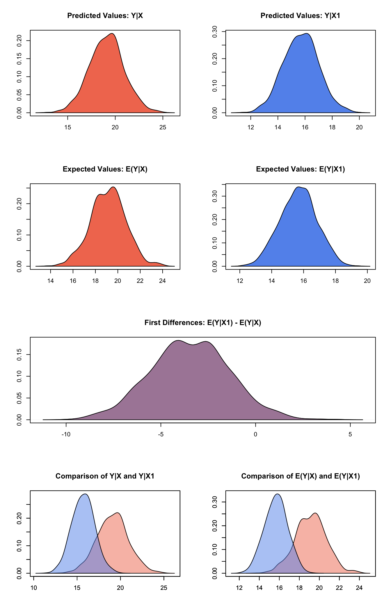
Graphs of Quantities of Interest for Quantile Regression
Using Dummy Variables
We can estimate a model of unemployment as a function of macroeconomic indicators and fixed effects for each country (see for help with dummy variables). Note that you do not need to create dummy variables, as the program will automatically parse the unique values in the selected variable into discrete levels.
data(macro)
z.out2 <- zelig(unem ~ gdp + trade + capmob + as.factor(country),
                model = "rq", tau = 0.5,
                data = macro)
## How to cite this model in Zelig:
## Alexander D'Amour. 2008.
## quantile: Quantile Regression for Continuous Dependent Variables
## in Christine Choirat, Christopher Gandrud, James Honaker, Kosuke Imai, Gary King, and Olivia Lau,
## "Zelig: Everyone's Statistical Software," http://zeligproject.org/Set values for the explanatory variables, using the default mean/mode values, with country set to the United States and Japan, respectively:
Simulate quantities of interest:
s.out2 <- sim(z.out2, x = x.US, x1 = x.Japan)summary(s.out2)##
## sim x :
## -----
## ev
## mean sd 50% 2.5% 97.5%
## 1 11.60458 0.6092805 11.58133 10.4415 12.76068
## pv
## mean sd 50% 2.5% 97.5%
## 1 11.60311 0.609773 11.5698 10.43624 12.76432
##
## sim x1 :
## -----
## ev
## mean sd 50% 2.5% 97.5%
## 1 6.854616 0.4038854 6.849454 6.084071 7.646943
## pv
## mean sd 50% 2.5% 97.5%
## 1 6.854618 0.4035154 6.84879 6.087191 7.649128
## fd
## mean sd 50% 2.5% 97.5%
## 1 -4.749969 0.4232467 -4.746332 -5.561712 -3.946614plot(s.out2)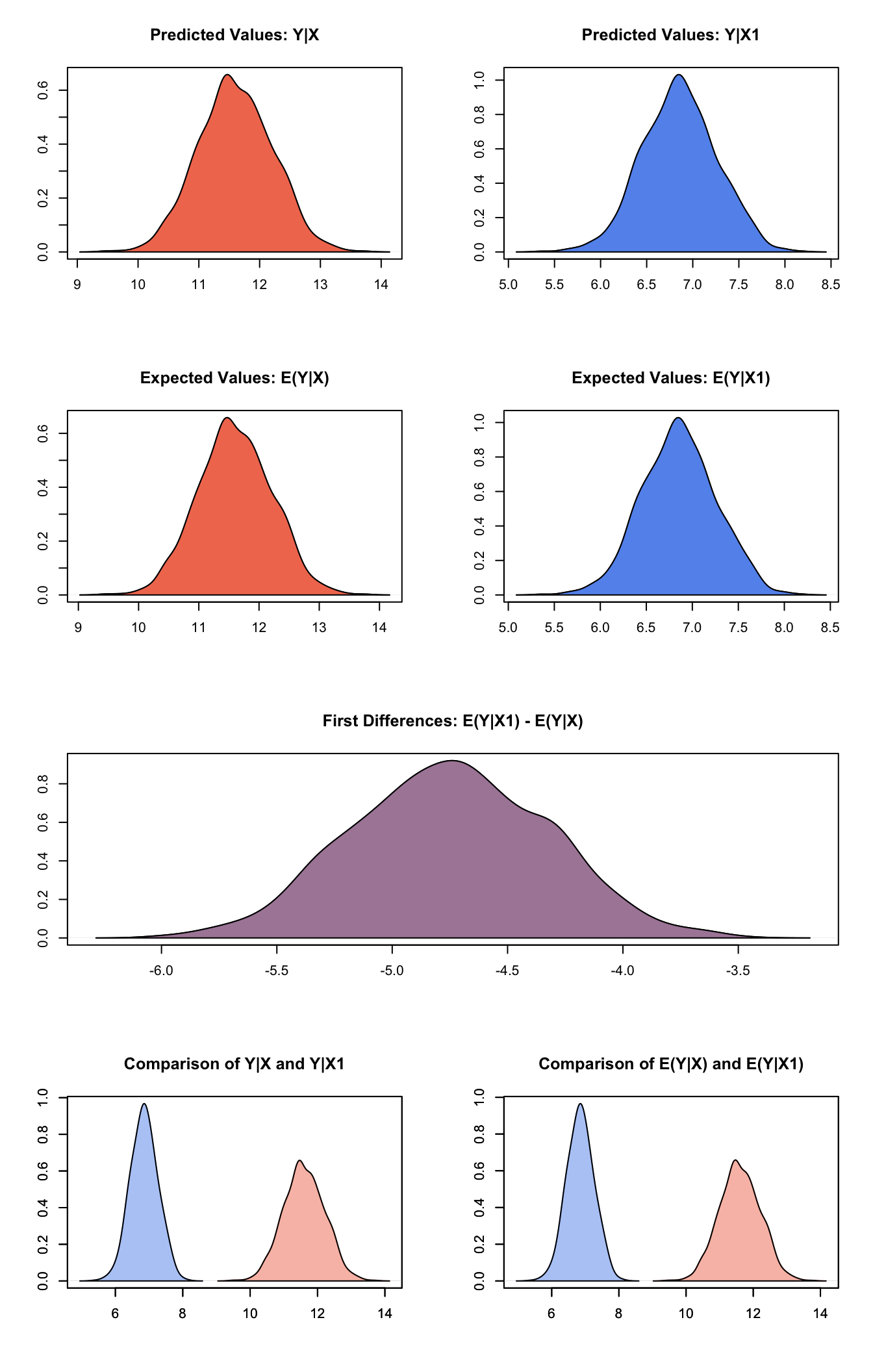
Graphs of Quantities of Interest for Quantile Regression
Estimating Multiple Quantiles
Using the Engel dataset (from the quantreg package) on food expenditure as a function of income, we can use the “quantile” model to estimate multiple conditional quantiles:
data(engel, package="quantreg")
z.out3 <- zelig(foodexp ~ income, model = "rq",
                tau = seq(0.1, 0.9, by = 0.1), data = engel)
We can summarize the coefficient fits, or plot them to compare them to the least squares conditional mean estimator.
summary(z.out3)plot(summary(z.out3))Set the value of income to the top quartile and the bottom quartile of the income distribution for each fit:
x.bottom <- setx(z.out3, income = quantile(engel$income, 0.25))
x.top <- setx(z.out3, income = quantile(engel$income, 0.75))
Simulate quantities of interest for each fit simultaneously:
s.out3 <- sim(z.out3, x = x.bottom, x1 = x.top)Summary
summary(s.out3)Model
The quantile estimator is best introduced by considering the sample median estimator and comparing it to the sample mean estimator. To find the mean of a sample, we solve for the quantity \(\mu\) which minimizes the sum squared residuals:
\[ \begin{aligned} \mu &=& \arg\min_\mu \sum_i (y_i-\mu)^2\end{aligned} \]
Estimating a quantile is similar, but we solve for \(\xi\) which minimizes the sum absolute residuals:
\[ \begin{aligned} \xi &=& \arg\min_\xi \sum_i |y_i-\xi| \end{aligned} \]
One can confirm the equivalence of these optimization problems and the standard mean and median operators by taking the derivative with respect to the argument and setting it to zero.
The relationship between quantile regression and ordinary least squares regression is analogous to the relationship between the sample median and the sample mean, except we are now solving for the conditional median or conditional mean given covariates and a linear functional form. The optimization problems for the sample mean and median are then easily generalized to optimization problems for estimating conditional means or medians by replacing \(\mu\) or \(\xi\) with a linear combination of covariates \(X'\beta\):
\[ \begin{aligned} \hat\beta_\mathrm{mean} &=& \arg\min_\beta \sum_i (Y_i-X_i'\beta)^2 \nonumber \\ \hat\beta_\mathrm{median} &=& \arg\min_\beta \sum_i |Y_i-X_i'\beta| \label{median} \end{aligned} \]
Equation [median] can be generalized to provide any quantile of the conditional distribution, not just the median. We do this by weighting the aboslute value function asymmetrically in proportion to the requested \(\tau\) th quantile:
\[ \begin{aligned} \hat\beta_{\tau} &=& \arg\max_\beta \sum \rho(Y_i-X_i'\beta) \label{beta}\\ \rho &=& \tau(1-I(Y-X_i'\beta > 0)) + (1-\tau)I(Y-X_i'\beta > 0) \nonumber \end{aligned} \]
We call the asymmetric absolute value function a “check function”. This optimization problem has no closed form solution and is solved via linear programming.
Equation [beta] now lets us define a conditional quantile estimator. Suppose that for a given set of covariates \(x\), the response variable \(Y\) has as true conditional probability distribution \(f(\theta | x)\) where \(f\) can be any probability density function parametrized by a vector of parameters \(\theta\). This density function defines a value \(Q_\tau(\theta|x)\), the true \(\tau\) th population quantile given \(x\). We can write our conditional quantile estimator \(\hat Q_\tau(\theta|x)\) as:
\[ \begin{aligned} \hat Q_\tau(\theta|x) &=& x'\hat\beta_\tau \end{aligned} \]
Where \(\hat\beta\) is the vector that solves equation [beta]. Because we solve for the estimator \(\hat Q_\tau\) without constructing a likelihood function, it is not straightforward to specify a systematic and stochastic component for conditional quantile estimates. However, systematic and stochastic components do emerge asymptotically in the large- \(n\) limit. Asymptotically, \(\hat Q_\tau\) is normally distributed, and can be written with stochastic component
\[ \begin{aligned} \hat Q_\tau &\sim& \mathcal{N}(\mu, \sigma^2), \end{aligned} \]
And systematic components
\[ \begin{aligned} \mu &=& x'\hat\beta_\tau\\ \sigma^2 &=& \frac{\tau(1-\tau)}{n f^2}, \end{aligned} \]
Where \(n\) is the number of datapoints, and \(f\) is the true population density at the \(\tau\) th conditional quantile. Zelig uses this asymptotic approximation of stochastic and systematic components in simulation and numerically estimates the population density to derive \(\sigma^2\). The simulation results should thus be treated with caution when using small datasets as both this asymptotic approximation and the population density approximation can break down.
Quantities of Interest
- The expected value (
qi$ev) is the mean of simulations from the stochastic component,
\[ E(\hat Q_\tau) = x_i \beta_\tau, \]
given a draw of \(\beta_\tau\) from its sampling distribution. Variation in the expected value distribution comes from estimation uncertainty of \(\beta_\tau\).
The predicted value (
qi$pr) is the result of a single draw from the stochastic component given a draw of \(\beta_\tau\) from its sampling distribution. The distribution of predicted values should be centered around the same place as the expected values but have larger variance because it includes both estimation uncertainty and fundamental uncertainty.This model does not support conditional prediction.
Output Values
The Zelig object stores fields containing everything needed to rerun the Zelig output, and all the results and simulations as they are generated. In addition to the summary commands demonstrated above, some simply utility functions (known as getters) provide easy access to the raw fields most commonly of use for further investigation.
In the example above z.out$get_coef() returns the estimated coefficients, z.out$get_vcov() returns the estimated covariance matrix, and z.out$get_predict() provides predicted values for all observations in the dataset from the analysis.
See also
The quantile regression package quantreg by Richard Koenker. In addition, advanced users may wish to refer to help(rq), help(summary.rq) and help(rq.object).
Koenker R (2017). quantreg: Quantile Regression. R package version 5.33, <URL: https://CRAN.R-project.org/package=quantreg>.