Tobit
2017-10-29
Built using Zelig version 5.1.4.90000
Linear Regression for a Left-Censored Dependent Variable with tobit.
Tobit regression estimates a linear regression model for a left-censored dependent variable, where the dependent variable is censored from below. While the classical tobit model has values censored at 0, you may select another censoring point. For other linear regression models with fully observed dependent variables, see Bayesian regression, maximum likelihood normal regression, and least squares.
Inputs
zelig() accepts the following arguments to specify how the dependent variable is censored.
below: (defaults to 0) The point at which the dependent variable is censored from below. If any values in the dependent variable are observed to be less than the censoring point, it is assumed that that particular observation is censored from below at the observed value. (See also the Bayesian implementation which supports both left and right censoring.)robust: defaults to FALSE. If TRUE, zelig() computes robust standard errors based on sandwich estimators (see and ) and the options selected in cluster.cluster: if robust = TRUE, you may select a variable to define groups of correlated observations. Let x3 be a variable that consists of either discrete numeric values, character strings, or factors that define strata. Then
z.out <- zelig(y ~ x1 + x2, robust = TRUE, cluster = "x3",
                        model = "tobit", data = mydata)
means that the observations can be correlated within the strata defined by the variable x3, and that robust standard errors should be calculated according to those clusters. If robust = TRUE but cluster is not specified, zelig() assumes that each observation falls into its own cluster.
Zelig users may wish to refer to help(survreg) for more information.
Examples
Basic Example
Attaching the sample dataset:
data(tobin)Estimating linear regression using tobit:
z.out <- zelig(durable ~ age + quant, model = "tobit", data = tobin)## How to cite this model in Zelig:
## Christian Kleiber, and Achim Zeileis. 2011.
## tobit: Linear regression for Left-Censored Dependent Variable
## in Christine Choirat, Christopher Gandrud, James Honaker, Kosuke Imai, Gary King, and Olivia Lau,
## "Zelig: Everyone's Statistical Software," http://zeligproject.org/Summarize estimated paramters:
summary(z.out)## Model:
##
## Call:
## z5$zelig(formula = durable ~ age + quant, data = tobin)
##
## Observations:
## Total Left-censored Uncensored Right-censored
## 20 13 7 0
##
## Coefficients:
## Estimate Std. Error z value Pr(>|z|)
## (Intercept) 15.14487 16.07945 0.942 0.346
## age -0.12906 0.21858 -0.590 0.555
## quant -0.04554 0.05825 -0.782 0.434
## Log(scale) 1.71785 0.31032 5.536 3.1e-08
##
## Scale: 5.573
##
## Gaussian distribution
## Number of Newton-Raphson Iterations: 3
## Log-likelihood: -28.94 on 4 Df
## Wald-statistic: 1.124 on 2 Df, p-value: 0.57002
##
## Next step: Use 'setx' methodSetting values for the explanatory variables to their sample averages:
x.out <- setx(z.out)Simulating quantities of interest from the posterior distribution given x.out.
s.out1 <- sim(z.out, x = x.out)summary(s.out1)##
## sim x :
## -----
## ev
## mean sd 50% 2.5% 97.5%
## 1 1.534273 0.6350075 1.451001 0.5103966 3.042459
## pv
## mean sd 50% 2.5% 97.5%
## [1,] 3.002031 4.027547 1.310886 0 13.19713Simulating First Differences
Set explanatory variables to their default(mean/mode) values, with high (80th percentile) and low (20th percentile) liquidity ratio (quant):
x.high <- setx(z.out, quant = quantile(tobin$quant, prob = 0.8))
x.low <- setx(z.out, quant = quantile(tobin$quant, prob = 0.2))
Estimating the first difference for the effect of high versus low liquidity ratio on duration( durable):
s.out2 <- sim(z.out, x = x.high, x1 = x.low)summary(s.out2)##
## sim x :
## -----
## ev
## mean sd 50% 2.5% 97.5%
## 1 1.167931 0.7337131 1.030031 0.1629001 2.929642
## pv
## mean sd 50% 2.5% 97.5%
## [1,] 2.808371 4.002763 0.9649713 0 13.53341
##
## sim x1 :
## -----
## ev
## mean sd 50% 2.5% 97.5%
## 1 2.037927 0.9616189 1.909788 0.5752316 4.217732
## pv
## mean sd 50% 2.5% 97.5%
## [1,] 3.670113 4.446672 2.242544 0 15.69732
## fd
## mean sd 50% 2.5% 97.5%
## 1 0.8699962 1.166879 0.8246356 -1.335144 3.159152plot(s.out1)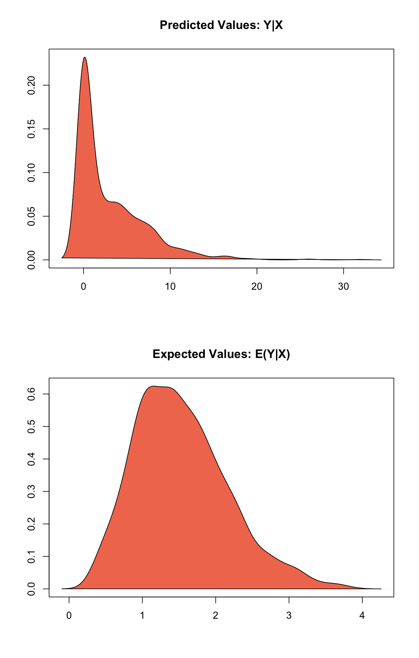
Graphs of Quantities of Interest for Zelig-tobit
Model
- Let \(Y_i^*\) be a latent dependent variable which is distributed with stochastic component
\[ \begin{aligned} Y_i^* & \sim & \textrm{Normal}(\mu_i, \sigma^2) \\\end{aligned} \]
where \(\mu_i\) is a vector means and \(\sigma^2\) is a scalar variance parameter. \(Y_i^*\) is not directly observed, however. Rather we observed \(Y_i\) which is defined as:
\[ Y_i = \left\{ \begin{array}{lcl} Y_i^* &\textrm{if} & c <Y_i^* \\ c &\textrm{if} & c \ge Y_i^* \end{array}\right. \]
where \(c\) is the lower bound below which \(Y_i^*\) is censored.
- The systematic component is given by
\[ \begin{aligned} \mu_{i} &=& x_{i} \beta,\end{aligned} \]
where \(x_{i}\) is the vector of \(k\) explanatory variables for observation \(i\) and \(\beta\) is the vector of coefficients.
Quantities of Interest
- The expected values (
qi$ev) for the tobit regression model are the same as the expected value of \(Y*\):
\[ E(Y^* | X) = \mu_{i} = x_{i} \beta \]
- The first difference (
qi$fd) for the tobit regression model is defined as
\[ \begin{aligned} \text{FD}=E(Y^* \mid x_{1}) - E(Y^* \mid x).\end{aligned} \]
- In conditional prediction models, the average expected treatment effect (
qi$att.ev) for the treatment group is
\[ \begin{aligned} \frac{1}{\sum t_{i}}\sum_{i:t_{i}=1}[E[Y^*_{i}(t_{i}=1)]-E[Y^*_{i}(t_{i}=0)]],\end{aligned} \]
where \(t_{i}\) is a binary explanatory variable defining the treatment (\(t_{i}=1\)) and control (\(t_{i}=0\)) groups.
Output Values
The Zelig object stores fields containing everything needed to rerun the Zelig output, and all the results and simulations as they are generated. In addition to the summary commands demonstrated above, some simply utility functions (known as getters) provide easy access to the raw fields most commonly of use for further investigation.
In the example above z.out$get_coef() returns the estimated coefficients, z.out$get_vcov() returns the estimated covariance matrix, and z.out$get_predict() provides predicted values for all observations in the dataset from the analysis.
See also
The tobit function is part of the survival library by Terry Therneau, ported to R by Thomas Lumley. Advanced users may wish to refer to help(survfit) in the survival library.
Kleiber C and Zeileis A (2008). Applied Econometrics with R. Springer-Verlag, New York. ISBN 978-0-387-77316-2, <URL: https://CRAN.R-project.org/package=AER>.