Bivariate Logistic Regression

Built using Zelig version 5.1.4.90000

Bivariate Logistic Regression for Two Dichotomous Dependent Variables with blogit from ZeligChoice.

Use the bivariate logistic regression model if you have two binary dependent variables $(Y_1, Y_2)$, and wish to model them jointly as a function of some explanatory variables. Each pair of dependent variables $(Y_{i1}, Y_{i2})$ has four potential outcomes, $(Y_{i1}=1, Y_{i2}=1)$, $(Y_{i1}=1, Y_{i2}=0)$, $(Y_{i1}=0, Y_{i2}=1)$, and $(Y_{i1}=0, Y_{i2}=0)$. The joint probability for each of these four outcomes is modeled with three systematic components: the marginal Pr $(Y_{i1} = 1)$ and Pr $(Y_{i2} = 1)$, and the odds ratio $\psi$, which describes the dependence of one marginal on the other. Each of these systematic components may be modeled as functions of (possibly different) sets of explanatory variables.

Syntax

First load packages:

library(zeligverse)

z.out <- zelig(cbind(Y1, Y2) ~ X1 + X2 + X3,
               model = "blogit", data = mydata)
x.out <- setx(z.out)
s.out <- sim(z.out, x = x.out, x1 = NULL)

Input Values

In every bivariate logit specification, there are three equations which correspond to each dependent variable ($Y_1$, $Y_2$), and $\psi$, the odds ratio. You should provide a list of formulas for each equation or, you may use cbind() if the right hand side is the same for both equations

formulae <- list(cbind(Y1, Y2),   X1 + X2)

which means that all the explanatory variables in equations 1 and 2 (corresponding to $Y_1$ and $Y_2$) are included, but only an intercept is estimated (all explanatory variables are omitted) for equation 3 ($\psi$).

Anticipated feature, not currently enabled:

You may use the function tag() to constrain variables across equations:

formulae <- list(mu1 = y1   x1 + tag(x3, "x3"), mu2 = y2 ~ x2 + tag(x3, "x3"))

where tag() is a special function that constrains variables to have the same effect across equations. Thus, the coefficient for x3 in equation mu1 is constrained to be equal to the coefficient for x3 in equation mu2.

Examples

Basic Example

Load the data and estimate the model:

data(sanction)

z.out1 <- zelig(cbind(import, export) ~ coop + cost + target,
                model = "blogit", data = sanction)

## How to cite this model in Zelig:
##   Thomas W. Yee. 2007.
##   blogit: Bivariate Logit Regression for Dichotomous Dependent Variables
##   in Christine Choirat, Christopher Gandrud, James Honaker, Kosuke Imai, Gary King, and Olivia Lau,
##   "Zelig: Everyone's Statistical Software," http://zeligproject.org/

summary(z.out1)

## Model: 
## 
## Call:
## z5$zelig(formula = cbind(import, export) ~ coop + cost + target, 
##     data = sanction)
## 
## 
## Pearson residuals:
##                 Min      1Q   Median     3Q   Max
## logit(mu1)   -2.184 -0.5255 -0.27618 0.4669 2.112
## logit(mu2)   -4.924 -0.4599  0.08869 0.6242 3.079
## loge(oratio) -2.122 -0.4145  0.09651 0.2451 4.750
## 
## Coefficients: 
##               Estimate Std. Error z value Pr(>|z|)
## (Intercept):1 -2.88048    1.09504  -2.630 0.008527
## (Intercept):2 -3.28639    1.05862  -3.104 0.001907
## (Intercept):3 -0.63660    0.73944  -0.861 0.389283
## coop:1         0.28705    0.33854   0.848 0.396501
## coop:2        -0.06214    0.33798  -0.184 0.854117
## cost:1         2.43481    0.66010   3.689 0.000226
## cost:2         2.72058    0.70009   3.886 0.000102
## target:1      -1.23994    0.48258  -2.569 0.010188
## target:2      -0.49957    0.44868  -1.113 0.265533
## 
## Number of linear predictors:  3 
## 
## Names of linear predictors: logit(mu1), logit(mu2), loge(oratio)
## 
## Residual deviance: 143.9813 on 225 degrees of freedom
## 
## Log-likelihood: -71.9906 on 225 degrees of freedom
## 
## Number of iterations: 8 
## 
## Odds ratio:  0.5291 
## Next step: Use 'setx' method

By default, zelig() estimates two effect parameters for each explanatory variable in addition to the odds ratio parameter; this formulation is parametrically independent (estimating unconstrained effects for each explanatory variable), but stochastically dependent because the models share an odds ratio. Generate baseline values for the explanatory variables (with cost set to 1, net gain to sender) and alternative values (with cost set to 4, major loss to sender):

x.low <- setx(z.out1, cost = 1)
x.high <- setx(z.out1, cost = 4)

Simulate fitted values and first differences:

s.out1 <- sim(z.out1, x = x.low, x1 = x.high)

summary(s.out1)

## 
##  sim x :
##  -----
## ev
##                       mean          sd         50%         2.5%      97.5%
## Pr(Y1=0, Y2=0) 0.764861591 0.076898592 0.772636018 0.5944076854 0.88725505
## Pr(Y1=0, Y2=1) 0.154020913 0.070016048 0.142438021 0.0489447680 0.31276532
## Pr(Y1=1, Y2=0) 0.072289227 0.042523632 0.063896509 0.0181190387 0.17905193
## Pr(Y1=1, Y2=1) 0.008828269 0.008855768 0.006083191 0.0009329502 0.03424973
## pv
##                  0     1
## (Y1=0, Y2=0) 0.228 0.772
## (Y1=0, Y2=1) 0.862 0.138
## (Y1=1, Y2=0) 0.922 0.078
## (Y1=1, Y2=1) 0.988 0.012
## 
##  sim x1 :
##  -----
## ev
##                        mean           sd          50%         2.5%
## Pr(Y1=0, Y2=0) 6.764547e-05 0.0002870721 8.479136e-06 1.122442e-07
## Pr(Y1=0, Y2=1) 2.285438e-02 0.0381670056 8.975354e-03 5.498571e-04
## Pr(Y1=1, Y2=0) 5.892645e-03 0.0157226985 1.655853e-03 6.435737e-05
## Pr(Y1=1, Y2=1) 9.711853e-01 0.0402994376 9.849211e-01 8.690317e-01
##                       97.5%
## Pr(Y1=0, Y2=0) 0.0005593426
## Pr(Y1=0, Y2=1) 0.1159743052
## Pr(Y1=1, Y2=0) 0.0362570809
## Pr(Y1=1, Y2=1) 0.9983926520
## pv
##                  0     1
## (Y1=0, Y2=0) 1.000 0.000
## (Y1=0, Y2=1) 0.984 0.016
## (Y1=1, Y2=0) 0.991 0.009
## (Y1=1, Y2=1) 0.025 0.975
## fd
##                       mean         sd         50%       2.5%        97.5%
## Pr(Y1=0, Y2=0) -0.76479395 0.07698080 -0.77262061 -0.8872549 -0.594345342
## Pr(Y1=0, Y2=1) -0.13116653 0.08268646 -0.12371949 -0.3046665  0.011741846
## Pr(Y1=1, Y2=0) -0.06639658 0.04707685 -0.05916388 -0.1759960 -0.001374144
## Pr(Y1=1, Y2=1)  0.96235706 0.04459420  0.97703091  0.8535263  0.996593467

plot(s.out1)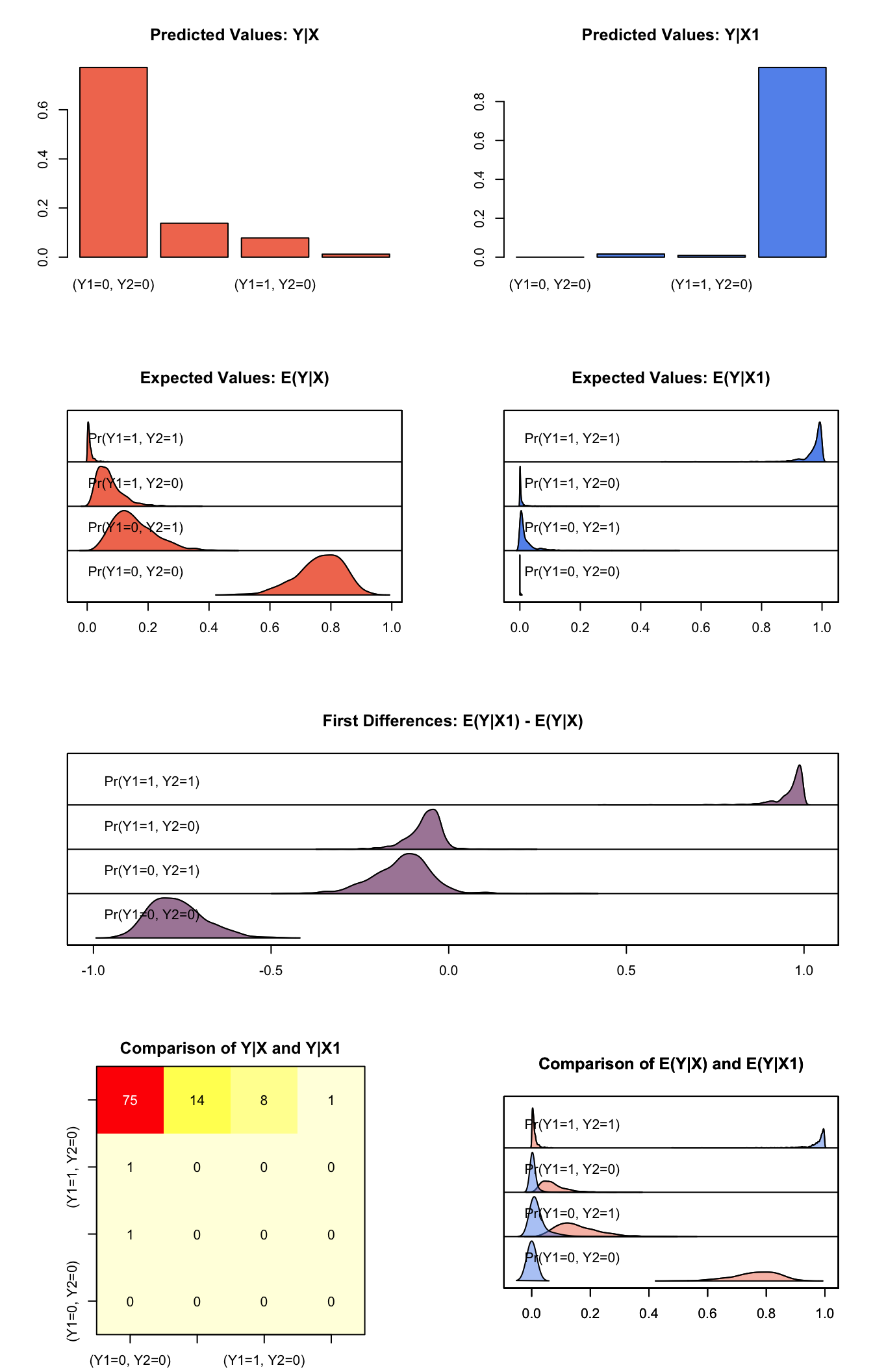

Graphs of Quantities of Interest for Bivariate Logit

Model

For each observation, define two binary dependent variables, $Y_1$ and $Y_2$, each of which take the value of either 0 or 1 (in the following, we suppress the observation index). We model the joint outcome $(Y_1$, $Y_2)$ using a marginal probability for each dependent variable, and the odds ratio, which parameterizes the relationship between the two dependent variables. Define $Y_{rs}$ such that it is equal to 1 when $Y_1=r$ and $Y_2=s$ and is 0 otherwise, where $r$ and $s$ take a value of either 0 or 1. Then, the model is defined as follows,

The stochastic component is

\[ \begin{aligned} Y_{11} &\sim& \textrm{Bernoulli}(y_{11} \mid \pi_{11}) \\ Y_{10} &\sim& \textrm{Bernoulli}(y_{10} \mid \pi_{10}) \\ Y_{01} &\sim& \textrm{Bernoulli}(y_{01} \mid \pi_{01}) \end{aligned} \]

where $\pi_{rs}=\Pr(Y_1=r, Y_2=s)$ is the joint probability, and $\pi_{00}=1-\pi_{11}-\pi_{10}-\pi_{01}$.

The systematic components model the marginal probabilities, $\pi_j=\Pr(Y_j=1)$, as well as the odds ratio. The odds ratio is defined as $\psi = \pi_{00} \pi_{01}/\pi_{10}\pi_{11}$ and describes the relationship between the two outcomes. Thus, for each observation we have

\[ \begin{aligned} \pi_j & = & \frac{1}{1 + \exp(-x_j \beta_j)} \quad \textrm{ for} \quad j=1,2, \\ \psi &= & \exp(x_3 \beta_3). \end{aligned} \]

Quantities of Interest

The expected values (qi$ev) for the bivariate logit model are the predicted joint probabilities. Simulations of $\beta_1$, $\beta_2$, and $\beta_3$ (drawn from their sampling distributions) are substituted into the systematic components $(\pi_1, \pi_2, \psi)$ to find simulations of the predicted joint probabilities:

\[ \begin{aligned} \pi_{11} & = & \left\{ \begin{array}{ll} \frac{1}{2}(\psi - 1)^{-1} - {a - \sqrt{a^2 + b}} & \textrm{for} \; \psi \ne 1 \\ \pi_1 \pi_2 & \textrm{for} \; \psi = 1 \end{array} \right., \\ \pi_{10} &=& \pi_1 - \pi_{11}, \\ \pi_{01} &=& \pi_2 - \pi_{11}, \\ \pi_{00} &=& 1 - \pi_{10} - \pi_{01} - \pi_{11}, \end{aligned} \]

where $a = 1 + (\pi_1 + \pi_2)(\psi - 1)$, $b = -4 \psi(\psi - 1) \pi_1 \pi_2$, and the joint probabilities for each observation must sum to one. For $n$ simulations, the expected values form an $n \times 4$ matrix for each observation in x.

The predicted values (qi$pr) are draws from the multinomial distribution given the expected joint probabilities.
The first differences (qi$fd) for each of the predicted joint probabilities are given by

\[ \textrm{FD}_{rs} = \Pr(Y_1=r, Y_2=s \mid x_1)-\Pr(Y_1=r, Y_2=s \mid x). \]

The risk ratio (qi$rr) for each of the predicted joint probabilities are given by

\[ \textrm{RR}_{rs} = \frac{\Pr(Y_1=r, Y_2=s \mid x_1)}{\Pr(Y_1=r, Y_2=s \mid x)} \]

In conditional prediction models, the average expected treatment effect (att.ev) for the treatment group is

\[ \frac{1}{\sum_{i=1}^n t_i}\sum_{i:t_i=1}^n \left\{ Y_{ij}(t_i=1) - E[Y_{ij}(t_i=0)] \right\} \textrm{ for } j = 1,2, \]

where $t_i$ is a binary explanatory variable defining the treatment ($t_i=1$) and control ($t_i=0$) groups. Variation in the simulations are due to uncertainty in simulating $E[Y_{ij}(t_i=0)]$, the counterfactual expected value of $Y_{ij}$ for observations in the treatment group, under the assumption that everything stays the same except that the treatment indicator is switched to $t_i=0$.

In conditional prediction models, the average predicted treatment effect (att.pr) for the treatment group is

\[ \frac{1}{\sum_{i=1}^n t_i}\sum_{i:t_i=1}^n \left\{ Y_{ij}(t_i=1) - \widehat{Y_{ij}(t_i=0)} \right\} \textrm{ for } j = 1,2, \]

where $t_i$ is a binary explanatory variable defining the treatment ($t_i=1$) and control ($t_i=0$) groups. Variation in the simulations are due to uncertainty in simulating $\widehat{Y_{ij}(t_i=0)}$, the counterfactual predicted value of $Y_{ij}$ for observations in the treatment group, under the assumption that everything stays the same except that the treatment indicator is switched to $t_i=0$.

Output Values

The output of each Zelig command contains useful information which you may view. For example, if you run z.out <- zelig(y ~ x, model = "blogit", data), then you may examine the available information in z.out by using names(z.out), see the coefficients by using z.out$coefficients, and obtain a default summary of information through summary(z.out). Other elements available through the $ operator are listed below.

From the zelig() output object z.out, you may extract:
coefficients: the named vector of coefficients.
fitted.values: an $n \times 4$ matrix of the in-sample fitted values.
predictors: an $n \times 3$ matrix of the linear predictors $x_j \beta_j$.
residuals: an $n \times 3$ matrix of the residuals.
df.residual: the residual degrees of freedom.
df.total: the total degrees of freedom.
rss: the residual sum of squares.
y: an $n \times 2$ matrix of the dependent variables.
zelig.data: the input data frame if save.data = TRUE.
From summary(z.out), you may extract:
coef3: a table of the coefficients with their associated standard errors and $t$-statistics.
cov.unscaled: the variance-covariance matrix.
pearson.resid: an $n \times 3$ matrix of the Pearson residuals.

2017-10-29