Gamma Regression
2017-10-29
Built using Zelig version 5.1.4.90000
Gamma Regression for Continuous, Positive Dependent Variables with gamma.
Use the gamma regression model if you have a positive-valued dependent variable such as the number of years a parliamentary cabinet endures, or the seconds you can stay airborne while jumping. The gamma distribution assumes that all waiting times are complete by the end of the study (censoring is not allowed).
Example
Attach the sample data:
data(coalition)Estimate the model:
z.out <- zelig(duration ~ fract + numst2, model = "gamma", data = coalition)## How to cite this model in Zelig:
## R Core Team. 2007.
## gamma: Gamma Regression for Continuous, Positive Dependent Variables
## in Christine Choirat, Christopher Gandrud, James Honaker, Kosuke Imai, Gary King, and Olivia Lau,
## "Zelig: Everyone's Statistical Software," http://zeligproject.org/View the regression output:
summary(z.out)## Model:
##
## Call:
## z5$zelig(formula = duration ~ fract + numst2, data = coalition)
##
## Deviance Residuals:
## Min 1Q Median 3Q Max
## -2.2510 -0.9112 -0.2278 0.4132 1.5360
##
## Coefficients:
## Estimate Std. Error t value Pr(>|t|)
## (Intercept) -1.296e-02 1.329e-02 -0.975 0.33016
## fract 1.149e-04 1.723e-05 6.668 1.19e-10
## numst2 -1.739e-02 5.881e-03 -2.957 0.00335
##
## (Dispersion parameter for Gamma family taken to be 0.6291004)
##
## Null deviance: 300.74 on 313 degrees of freedom
## Residual deviance: 272.19 on 311 degrees of freedom
## AIC: 2428.1
##
## Number of Fisher Scoring iterations: 6
##
## Next step: Use 'setx' methodSet the baseline values (with the ruling coalition in the minority) and the alternative values (with the ruling coalition in the majority) for X:
Simulate expected values (qi$ev) and first differences (qi$fd):
s.out <- sim(z.out, x = x.low, x1 = x.high)summary(s.out)##
## sim x :
## -----
## ev
## mean sd 50% 2.5% 97.5%
## [1,] 14.4043 1.061457 14.33427 12.47827 16.6991
## pv
## mean sd 50% 2.5% 97.5%
## [1,] 13.86111 12.33949 10.67768 0.5294782 44.9441
##
## sim x1 :
## -----
## ev
## mean sd 50% 2.5% 97.5%
## [1,] 19.2101 1.090567 19.13691 17.2235 21.56033
## pv
## mean sd 50% 2.5% 97.5%
## [1,] 19.86033 18.47412 14.55303 1.020767 65.90548
## fd
## mean sd 50% 2.5% 97.5%
## [1,] 4.805793 1.499152 4.820032 1.881295 7.811935plot(s.out)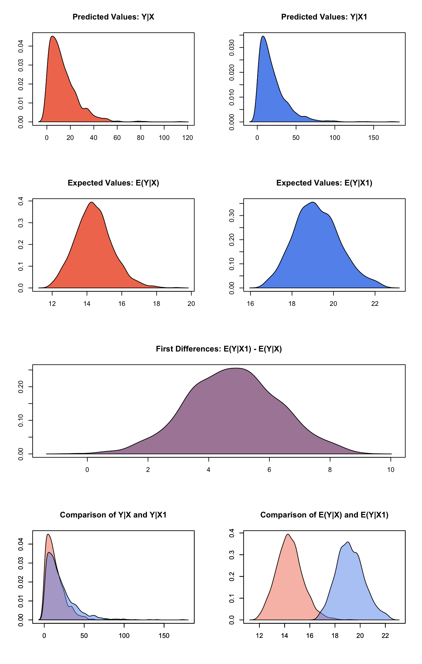
Graphs of Quantities of Interest for Zelig-gamma
Model
- The Gamma distribution with scale parameter \(\alpha\) has a stochastic component:
\[ \begin{aligned} Y &\sim& \textrm{Gamma}(y_i \mid \lambda_i, \alpha) \\ f(y) &=& \frac{1}{\alpha^{\lambda_i} \, \Gamma \lambda_i} \, y_i^{\lambda_i - 1} \exp -\left\{ \frac{y_i}{\alpha} \right\}\end{aligned} \] | for \(\alpha, \lambda_i, y_i > 0\).
- The systematic component is given by
\[ \lambda_i = \frac{1}{x_i \beta} \]
Quantities of Interest
- The expected values (qi$ev) are simulations of the mean of the stochastic component given draws of \(\alpha\) and \(\beta\) from their posteriors:
\[ E(Y) = \alpha \lambda_i. \]
The predicted values (qi$pr) are draws from the gamma distribution for each given set of parameters \((\alpha, \lambda_i)\).
If x1 is specified, sim() also returns the differences in the expected values (qi$fd),
\[ E(Y \mid x_1) - E(Y \mid x) \]
.
- In conditional prediction models, the average expected treatment effect (att.ev) for the treatment group is
\[ \frac{1}{\sum_{i=1}^n t_i}\sum_{i:t_i=1}^n \left\{ Y_i(t_i=1) - E[Y_i(t_i=0)] \right\}, \]
where \(t_i\) is a binary explanatory variable defining the treatment (\(t_i=1\)) and control (\(t_i=0\)) groups. Variation in the simulations are due to uncertainty in simulating \(E[Y_i(t_i=0)]\), the counterfactual expected value of \(Y_i\) for observations in the treatment group, under the assumption that everything stays the same except that the treatment indicator is switched to \(t_i=0\).
- In conditional prediction models, the average predicted treatment effect (att.pr) for the treatment group is
\[ \frac{1}{\sum_{i=1}^n t_i}\sum_{i:t_i=1}^n \left\{ Y_i(t_i=1) - \widehat{Y_i(t_i=0)} \right\}, \]
where \(t_i\) is a binary explanatory variable defining the treatment (\(t_i=1\)) and control (\(t_i=0\)) groups. Variation in the simulations are due to uncertainty in simulating \(\widehat{Y_i(t_i=0)}\), the counterfactual predicted value of \(Y_i\) for observations in the treatment group, under the assumption that everything stays the same except that the treatment indicator is switched to \(t_i=0\).
Output Values
The Zelig object stores fields containing everything needed to rerun the Zelig output, and all the results and simulations as they are generated. In addition to the summary commands demonstrated above, some simply utility functions (known as getters) provide easy access to the raw fields most commonly of use for further investigation.
In the example above z.out$get_coef() returns the estimated coefficients, z.out$get_vcov() returns the estimated covariance matrix, and z.out$get_predict() provides predicted values for all observations in the dataset from the analysis.
See also
The gamma model is part of the stats package by the R Core Team. Advanced users may wish to refer to help(glm) and help(family).
R Core Team (2017). R: A Language and Environment for Statistical Computing. R Foundation for Statistical Computing, Vienna, Austria. <URL: https://www.R-project.org/>.