Log-Normal
2017-10-29
Built using Zelig version 5.1.4.90000
Log-Normal Regression for Duration Dependent Variables with lognorm
The log-normal model describes an event’s duration, the dependent variable, as a function of a set of explanatory variables. The log-normal model may take time censored dependent variables, and allows the hazard rate to increase and decrease.
Syntax
z.out <- zelig(Surv(Y, C) ~ X, model = "lognorm", weights = w, data = mydata)
x.out <- setx(z.out)
s.out <- sim(z.out, x = x.out)
Log-normal models require that the dependent variable be in the form Surv(Y, C), where Y and C are vectors of length \(n\). For each observation \(i\) in 1, …, \(n\), the value \(y_i\) is the duration (lifetime, for example) of each subject, and the associated \(c_i\) is a binary variable such that \(c_i = 1\) if the duration is not censored (e.g., the subject dies during the study) or \(c_i = 0\) if the duration is censored (e.g., the subject is still alive at the end of the study). If \(c_i\) is omitted, all Y are assumed to be completed; that is, time defaults to 1 for all observations.
Input Values
In addition to the standard inputs, zelig() takes the following additional options for lognormal regression:
robust: defaults to FALSE. If TRUE, zelig() computes robust standard errors based on sandwich estimators (see and ) based on the options in cluster.
cluster: if robust = TRUE, you may select a variable to define groups of correlated observations. Let x3 be a variable that consists of either discrete numeric values, character strings, or factors that define strata. Then
z.out <- zelig(y ~ x1 + x2, robust = TRUE, cluster = "x3", model = "exp", data = mydata)means that the observations can be correlated within the strata defined by the variable x3, and that robust standard errors should be calculated according to those clusters. If robust = TRUE but cluster is not specified, zelig() assumes that each observation falls into its own cluster.
Example
Attach the sample data:
data(coalition)Estimate the model:
z.out <- zelig(Surv(duration, ciep12) ~ fract + numst2, model ="lognorm", data = coalition)## How to cite this model in Zelig:
## Terry M Therneau, and Thomas Lumley. 2007.
## lognorm: Log-Normal Regression for Duration Dependent Variables
## in Christine Choirat, Christopher Gandrud, James Honaker, Kosuke Imai, Gary King, and Olivia Lau,
## "Zelig: Everyone's Statistical Software," http://zeligproject.org/View the regression output:
summary(z.out)## Model:
##
## Call:
## z5$zelig(formula = Surv(duration, ciep12) ~ fract + numst2, data = coalition)
## Value Std. Error z p
## (Intercept) 5.36667 0.597517 8.98 2.67e-19
## fract -0.00444 0.000806 -5.51 3.65e-08
## numst2 0.55983 0.142351 3.93 8.40e-05
## Log(scale) 0.18239 0.044214 4.13 3.70e-05
##
## Scale= 1.2
##
## Log Normal distribution
## Loglik(model)= -1077.9 Loglik(intercept only)= -1101.2
## Chisq= 46.58 on 2 degrees of freedom, p= 7.7e-11
## Number of Newton-Raphson Iterations: 3
## n= 314
##
## Next step: Use 'setx' methodSet the baseline values (with the ruling coalition in the minority) and the alternative values (with the ruling coalition in the majority) for X:
Simulate expected values (qi\(ev) and first differences (qi\)fd):
s.out <- sim(z.out, x = x.low, x1 = x.high)summary(s.out)##
## sim x :
## -----
## ev
## mean sd 50% 2.5% 97.5%
## 1 18.28776 2.41547 18.17584 14.07644 23.433
## pv
## mean sd 50% 2.5% 97.5%
## [1,] 16.42204 23.98288 8.196013 0.8690616 83.68057
##
## sim x1 :
## -----
## ev
## mean sd 50% 2.5% 97.5%
## 1 31.89368 3.565827 31.73007 25.31423 39.38045
## pv
## mean sd 50% 2.5% 97.5%
## [1,] 33.06846 64.0542 15.65075 1.741425 162.7155
## fd
## mean sd 50% 2.5% 97.5%
## 1 13.60592 3.569912 13.46923 7.023056 20.70328plot(s.out)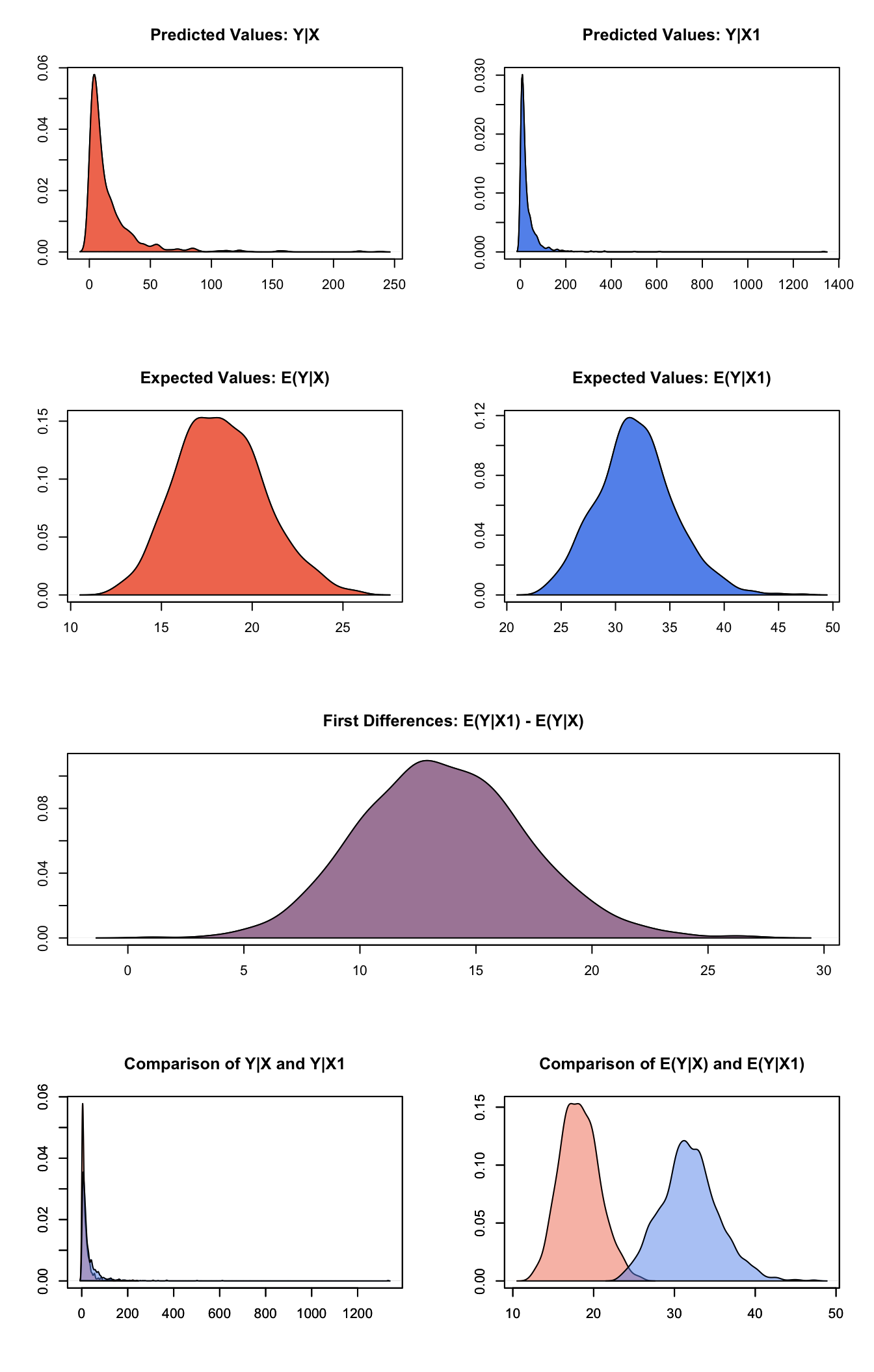
Graphs of Quantities of Interest for Zelig-lognorm
Model
Let \(Y_i^*\) be the survival time for observation \(i\) with the density function \(f(y)\) and the corresponding distribution function \(F(t)=\int_{0}^t f(y) dy\). This variable might be censored for some observations at a fixed time \(y_c\) such that the fully observed dependent variable, \(Y_i\), is defined as
\[ Y_i = \left\{ \begin{array}{ll} Y_i^* & \textrm{if }Y_i^* \leq y_c \\ y_c & \textrm{if }Y_i^* > y_c \\ \end{array} \right. \] - The stochastic component is described by the distribution of the partially observed variable, \(Y^*\). For the lognormal model, there are two equivalent representations:
\[ \begin{aligned} Y_i^* \; \sim \; \textrm{LogNormal}(\mu_i, \sigma^2) & \textrm{ or } & \log(Y_i^*) \; \sim \; \textrm{Normal}(\mu_i, \sigma^2)\end{aligned} \] where the parameters \(\mu_i\) and \(\sigma^2\) are the mean and variance of the Normal distribution. (Note that the output from zelig() parameterizes scale $ = $.)
In addition, survival models like the lognormal have three additional properties. The hazard function \(h(t)\) measures the probability of not surviving past time \(t\) given survival up to \(t\). In general, the hazard function is equal to \(f(t)/S(t)\) where the survival function \(S(t) =1 - \int_{0}^t f(s) ds\) represents the fraction still surviving at time \(t\). The cumulative hazard function \(H(t)\) describes the probability of dying before time \(t\). In general, \(H(t)= \int_{0}^{t} h(s) ds = -\log S(t)\). In the case of the lognormal model,
\[ \begin{aligned} h(t) &=& \frac{1}{\sqrt{2 \pi} \, \sigma t \, S(t)} \exp\left\{-\frac{1}{2 \sigma^2} (\log \lambda t)^2\right\} \\ S(t) &=& 1 - \Phi\left(\frac{1}{\sigma} \log \lambda t\right) \\ H(t) &=& -\log \left\{ 1 - \Phi\left(\frac{1}{\sigma} \log \lambda t\right) \right\}\end{aligned} \] where \(\Phi(\cdot)\) is the cumulative density function for the Normal distribution.
- The systematic component is described as:
\[ \mu_i = x_i \beta . \]
Quantities of Interest
- The expected values (qi$ev) for the lognormal model are simulations of the expected duration:
\[ E(Y) = \exp\left(\mu_i + \frac{1}{2}\sigma^2 \right), \]
given draws of \(\beta\) and \(\sigma\) from their sampling distributions.
The predicted value is a draw from the log-normal distribution given simulations of the parameters \((\lambda_i, \sigma)\).
The first difference (qi$fd) is
\[ \textrm{FD} = E(Y \mid x_1) - E(Y \mid x). \]
- In conditional prediction models, the average expected treatment effect (att.ev) for the treatment group is
\[ \frac{1}{\sum_{i=1}^n t_i}\sum_{i:t_i=1}^n \{ Y_i(t_i=1) - E[Y_i(t_i=0)] \}, \]
where \(t_i\) is a binary explanatory variable defining the treatment (\(t_i=1\)) and control (\(t_i=0\)) groups. When \(Y_i(t_i=1)\) is censored rather than observed, we replace it with a simulation from the model given available knowledge of the censoring process. Variation in the simulations is due to two factors: uncertainty in the imputation process for censored \(y_i^*\) and uncertainty in simulating \(E[Y_i(t_i=0)]\), the counterfactual expected value of \(Y_i\) for observations in the treatment group, under the assumption that everything stays the same except that the treatment indicator is switched to \(t_i=0\).
- In conditional prediction models, the average predicted treatment effect (att.pr) for the treatment group is
\[ \frac{1}{\sum_{i=1}^n t_i} \sum_{i:t_i=1}^n \{ Y_i(t_i=1) - \widehat{Y_i(t_i=0)} \}, \]
where \(t_i\) is a binary explanatory variable defining the treatment (\(t_i=1\)) and control (\(t_i=0\)) groups. When \(Y_i(t_i=1)\) is censored rather than observed, we replace it with a simulation from the model given available knowledge of the censoring process. Variation in the simulations are due to two factors: uncertainty in the imputation process for censored \(y_i^*\) and uncertainty in simulating \(\widehat{Y_i(t_i=0)}\), the counterfactual predicted value of \(Y_i\) for observations in the treatment group, under the assumption that everything stays the same except that the treatment indicator is switched to \(t_i=0\).
Output Values
The Zelig object stores fields containing everything needed to rerun the Zelig output, and all the results and simulations as they are generated. In addition to the summary commands demonstrated above, some simply utility functions (known as getters) provide easy access to the raw fields most commonly of use for further investigation.
In the example above z.out$get_coef() returns the estimated coefficients, z.out$get_vcov() returns the estimated covariance matrix, and z.out$get_predict() provides predicted values for all observations in the dataset from the analysis.
See also
The exponential function is part of the survival library by by Terry Therneau, ported to R by Thomas Lumley. Advanced users may wish to refer to help(survfit) in the survival library.
Therneau T (2015). A Package for Survival Analysis in S. version 2.38, <URL: https://CRAN.R-project.org/package=survival>.
Terry M. Therneau and Patricia M. Grambsch (2000). Modeling Survival Data: Extending the Cox Model. Springer, New York. ISBN 0-387-98784-3.