Normal GEE

Built using Zelig version 5.1.4.90000

Generalized Estimating Equation for Normal Regression with normal.gee.

The GEE normal estimates the same model as the standard normal regression. Unlike in normal regression, GEE normal allows for dependence within clusters, such as in longitudinal data, although its use is not limited to just panel data. The user must first specify a “working” correlation matrix for the clusters, which models the dependence of each observation with other observations in the same cluster. The “working” correlation matrix is a $T \times T$ matrix of correlations, where $T$ is the size of the largest cluster and the elements of the matrix are correlations between within-cluster observations. The appeal of GEE models is that it gives consistent estimates of the parameters and consistent estimates of the standard errors can be obtained using a robust “sandwich” estimator even if the “working” correlation matrix is incorrectly specified. If the “working” correlation matrix is correctly specified, GEE models will give more efficient estimates of the parameters. GEE models measure population-averaged effects as opposed to cluster-specific effects (See ).

Syntax

z.out <- zelig(Y ~ X1 + X2, model = "normal.gee",
                       id = "X3", weights = w, data = mydata)
x.out <- setx(z.out)
s.out <- sim(z.out, x = x.out)

where id is a variable which identifies the clusters. The data should be sorted by id and should be ordered within each cluster when appropriate.

Additional Inputs

robust: defaults to TRUE. If TRUE, consistent standard errors are estimated using a “sandwich” estimator.

Use the following arguments to specify the structure of the “working” correlations within clusters:

corstr: defaults to “independence”. It can take on the following arguments:
Independence (corstr = independence): ${\rm cor}(y_{it}, y_{it'})=0$, $\forall t, t'$ with $t\ne t'$. It assumes that there is no correlation within the clusters and the model becomes equivalent to standard normal regression. The “working” correlation matrix is the identity matrix.
Fixed (corstr = fixed): If selected, the user must define the “working” correlation matrix with the R argument rather than estimating it from the model.
Stationary $m$ dependent (corstr = stat_M_dep):

\[ {\rm cor}(y_{it}, y_{it'})=\left\{\begin{array}{ccc} \alpha_{|t-t'|} & {\rm if} & |t-t'|\le m \\ 0 & {\rm if} & |t-t'| > m \end{array}\right. \] If (corstr = stat_M_dep), you must also specify Mv = $m$, where $m$ is the number of periods $t$ of dependence. Choose this option when the correlations are assumed to be the same for observations of the same $|t-t'|$ periods apart for $|t-t'| \leq m$.

  Sample "working" correlation for Stationary 2 dependence ($Mv=2$)

\[ \left( \begin{array}{ccccc} 1 & \alpha_1 & \alpha_2 & 0 & 0 \\ \alpha_1 & 1 & \alpha_1 & \alpha_2 & 0 \\ \alpha_2 & \alpha_1 & 1 & \alpha_1 & \alpha_2 \\ 0 & \alpha_2 & \alpha_1 & 1 & \alpha_1 \\ 0 & 0 & \alpha_2 & \alpha_1 & 1 \end{array} \right) \]

Non-stationary $m$ dependent (corstr = non_stat_M_dep):

\[ {\rm cor}(y_{it}, y_{it'})=\left\{\begin{array}{ccc} \alpha_{tt'} & {\rm if} & |t-t'|\le m \\ 0 & {\rm if} & |t-t'| > m \end{array}\right. \]

  If (`corstr = non_stat_M_dep`), you must also specify `Mv` =
  $m$, where $m$ is the number of periods $t$ of
  dependence. This option relaxes the assumption that the
  correlations are the same for all observations of the same
  $|t-t'|$ periods apart.

  Sample "working" correlation for Non-stationary 2 dependence
  (Mv=2)

\[ \left( \begin{array}{ccccc} 1 & \alpha_{12} & \alpha_{13} & 0 & 0 \\ \alpha_{12} & 1 & \alpha_{23} & \alpha_{24} & 0 \\ \alpha_{13} & \alpha_{23} & 1 & \alpha_{34} & \alpha_{35} \\ 0 & \alpha_{24} & \alpha_{34} & 1 & \alpha_{45} \\ 0 & 0 & \alpha_{35} & \alpha_{45} & 1 \end{array} \right) \]

Exchangeable (corstr = exchangeable):

\[ {\rm cor}(y_{it}, y_{it'})=\alpha, \]

  $\forall t, t'$ with $t\ne t'$. Choose this option if the correlations are
  assumed to be the same for all observations within the cluster.

  Sample "working" correlation for Exchangeable

\[ \left( \begin{array}{ccccc} 1 & \alpha & \alpha & \alpha & \alpha \\ \alpha & 1 & \alpha & \alpha & \alpha \\ \alpha & \alpha & 1 & \alpha & \alpha \\ \alpha & \alpha & \alpha & 1 & \alpha \\ \alpha & \alpha & \alpha & \alpha & 1 \end{array} \right) \]

Stationary $m$ th order autoregressive (corstr = AR-M): If (corstr = AR-M), you must also specify Mv = $m$, where $m$ is the number of periods $t$ of dependence. For example, the first order autoregressive model (AR-1) implies ${\rm cor}(y_{it}, y_{it'})=\alpha^{|t-t'|}, \forall t, t'$ with $t\ne t'$. In AR-1, observation 1 and observation 2 have a correlation of $\alpha$. Observation 2 and observation 3 also have a correlation of $\alpha$. Observation 1 and observation 3 have a correlation of $\alpha^2$, which is a function of how 1 and 2 are correlated ($\alpha$) multiplied by how 2 and 3 are correlated ($\alpha$). Observation 1 and 4 have a correlation that is a function of the correlation between 1 and 2, 2 and 3, and 3 and 4, and so forth.

Sample “working” correlation for Stationary AR-1 (Mv=1)

\[ \left( \begin{array}{ccccc} 1 & \alpha & \alpha^2 & \alpha^3 & \alpha^4 \\ \alpha & 1 & \alpha & \alpha^2 & \alpha^3 \\ \alpha^2 & \alpha & 1 & \alpha & \alpha^2 \\ \alpha^3 & \alpha^2 & \alpha & 1 & \alpha \\ \alpha^4 & \alpha^3 & \alpha^2 & \alpha & 1 \end{array} \right) \]

Unstructured (corstr = unstructured): ${\rm cor}(y_{it}, y_{it'})=\alpha_{tt'}$, $\forall t, t'$ with $t\ne t'$. No constraints are placed on the correlations, which are then estimated from the data.
Mv: defaults to 1. It specifies the number of periods of correlation and only needs to be specified when corstr is stat\_M\_dep, non\_stat\_M\_dep, or AR-M.
R: defaults to NULL. It specifies a user-defined correlation matrix rather than estimating it from the data. The argument is used only when corstr is “fixed”. The input is a $T \times T$ matrix of correlations, where $T$ is the size of the largest cluster.

Examples

Example with AR-1 Dependence

Attaching the sample turnout dataset:

data(macro)

Estimating model and presenting summary:

z.out <- zelig(unem ~ gdp + capmob + trade, model =
                       "normal.gee", id = "country", data = macro, corstr = "AR-M")

## Warning in if (corstrv == -1) stop("invalid corstr."): the condition has
## length > 1 and only the first element will be used

## Warning in if (corstrv == 5) stop("need zcor matrix for userdefined
## corstr.") else zcor <- genZcor(clusz, : the condition has length > 1 and
## only the first element will be used

## Warning in if (corstrv == 1) return(matrix(0, 0, 0)): the condition has
## length > 1 and only the first element will be used

## Warning in if (corstrv == 6) alpha <- 1 else alpha <- rep(0, q): the
## condition has length > 1 and only the first element will be used

## How to cite this model in Zelig:
##   Patrick Lam. 2011.
##   normal-gee: General Estimating Equation for Normal Regression
##   in Christine Choirat, Christopher Gandrud, James Honaker, Kosuke Imai, Gary King, and Olivia Lau,
##   "Zelig: Everyone's Statistical Software," http://zeligproject.org/

summary(z.out)

## Model: 
## 
## Call:
## z5$zelig(formula = unem ~ gdp + capmob + trade, id = "country", 
##     corstr = "AR-M", data = macro)
## 
##  Coefficients:
##             Estimate  Std.err   Wald Pr(>|W|)
## (Intercept) -1.41796  1.52884  0.860   0.3537
## gdp         -0.12153  0.06656  3.334   0.0679
## capmob       0.89741  0.50257  3.189   0.0742
## trade        0.13328  0.02613 26.013 3.39e-07
## 
## Estimated Scale Parameters:
##             Estimate Std.err
## (Intercept)    16.64   4.054
## 
## Correlation: Structure = exchangeable ar1 unstructured userdefined fixed

## Warning in if (pmatch(x$corstr, "independence", 0) == 0) {: the condition
## has length > 1 and only the first element will be used

##   Link = identity 
## 
## Estimated Correlation Parameters:
##       Estimate Std.err
## alpha   0.8118  0.0429
## Number of clusters:   14   Maximum cluster size: 25 
## Next step: Use 'setx' method

Set explanatory variables to their default (mean/mode) values, with high (80th percentile) and low (20th percentile) values:

x.high <- setx(z.out, trade = quantile(macro$trade, 0.8))
x.low <- setx(z.out, trade = quantile(macro$trade, 0.2))

Generate first differences for the effect of high versus low trade on GDP:

s.out <- sim(z.out, x = x.high, x1 = x.low)
summary(s.out)

## 
##  sim x :
##  -----
## ev
##       mean    sd   50%  2.5% 97.5%
## [1,] 7.878 1.291 7.852 5.368 10.38
## pv
##       mean    sd   50%   2.5% 97.5%
## [1,] 8.722 16.55 8.385 -23.65 42.21
## 
##  sim x1 :
##  -----
## ev
##      mean     sd  50%   2.5% 97.5%
## [1,] 2.35 0.8822 2.36 0.6665 3.935
## pv
##       mean    sd   50%   2.5% 97.5%
## [1,] 2.208 17.16 2.188 -32.53 34.13
## fd
##        mean    sd    50%   2.5%  97.5%
## [1,] -5.528 1.044 -5.512 -7.575 -3.454

Generate a plot of quantities of interest:

plot(s.out)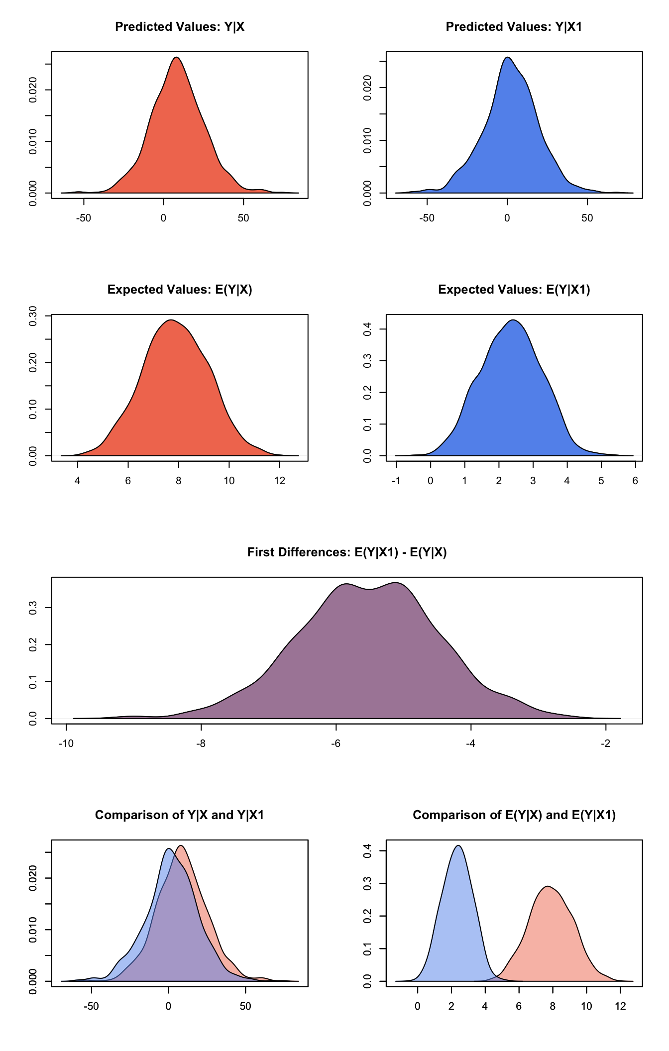

Graphs of Quantities of Interest for Normal GEE Model

The Model

Suppose we have a panel dataset, with $Y_{it}$ denoting the continuous dependent variable for unit $i$ at time $t$. $Y_{i}$ is a vector or cluster of correlated data where $y_{it}$ is correlated with $y_{it^\prime}$ for some or all $t, t^\prime$. Note that the model assumes correlations within $i$ but independence across $i$.

The stochastic component is given by the joint and marginal distributions

$$ \[\begin{aligned} Y_{i} &\sim& f(y_{i} \mid \mu_{i})\\ Y_{it} &\sim& g(y_{it} \mid \mu_{it}) \end{aligned}\]

where $f$ and $g$ are unspecified distributions with means $\mu_{i}$ and $\mu_{it}$. GEE models make no distributional assumptions and only require three specifications: a mean function, a variance function, and a correlation structure.

The systematic component is the mean function, given by:

\[ \mu_{it} = x_{it} \beta \]

where $x_{it}$ is the vector of $k$ explanatory variables for unit $i$ at time $t$ and $\beta$ is the vector of coefficients.

The variance function is given by:

\[ V_{it} = 1 \]

The correlation structure is defined by a $T \times T$ “working” correlation matrix, where $T$ is the size of the largest cluster. Users must specify the structure of the “working” correlation matrix a priori. The “working” correlation matrix then enters the variance term for each $i$, given by:

\[ V_{i} = \phi \, A_{i}^{\frac{1}{2}} R_{i}(\alpha) A_{i}^{\frac{1}{2}} \]

where $A_{i}$ is a $T \times T$ diagonal matrix with the variance function $V_{it} = 1$ as the $t$ th diagonal element (in the case of GEE normal, $A_{i}$ is the identity matrix), $R_{i}(\alpha)$ is the “working” correlation matrix, and $\phi$ is a scale parameter. The parameters are then estimated via a quasi-likelihood approach.

In GEE models, if the mean is correctly specified, but the variance and correlation structure are incorrectly specified, then GEE models provide consistent estimates of the parameters and thus the mean function as well, while consistent estimates of the standard errors can be obtained via a robust “sandwich” estimator. Similarly, if the mean and variance are correctly specified but the correlation structure is incorrectly specified, the parameters can be estimated consistently and the standard errors can be estimated consistently with the sandwich estimator. If all three are specified correctly, then the estimates of the parameters are more efficient.
The robust “sandwich” estimator gives consistent estimates of the standard errors when the correlations are specified incorrectly only if the number of units $i$ is relatively large and the number of repeated periods $t$ is relatively small. Otherwise, one should use the “naïve” model-based standard errors, which assume that the specified correlations are close approximations to the true underlying correlations. See for more details.

Quantities of Interest

All quantities of interest are for marginal means rather than joint means.
The method of bootstrapping generally should not be used in GEE models. If you must bootstrap, bootstrapping should be done within clusters, which is not currently supported in Zelig. For conditional prediction models, data should be matched within clusters.
The expected values (qi$ev) for the GEE normal model is the mean of simulations from the stochastic component:

\[ E(Y) = \mu_{c}= x_{c} \beta, \]

given draws of $\beta$ from its sampling distribution, where $x_{c}$ is a vector of values, one for each independent variable, chosen by the user.

The first difference (qi$fd) for the GEE normal model is defined as

\[ \textrm{FD} = \Pr(Y = 1 \mid x_1) - \Pr(Y = 1 \mid x). \]

In conditional prediction models, the average expected treatment effect (att.ev) for the treatment group is

\[ \frac{1}{\sum_{i=1}^n \sum_{t=1}^T tr_{it}}\sum_{i:tr_{it}=1}^n \sum_{t:tr_{it}=1}^T \left\{ Y_{it}(tr_{it}=1) - E[Y_{it}(tr_{it}=0)] \right\}, \]

where $tr_{it}$ is a binary explanatory variable defining the treatment ($tr_{it}=1$) and control ($tr_{it}=0$) groups. Variation in the simulations are due to uncertainty in simulating $E[Y_{it}(tr_{it}=0)]$, the counterfactual expected value of $Y_{it}$ for observations in the treatment group, under the assumption that everything stays the same except that the treatment indicator is switched to $tr_{it}=0$.

Output Values

The output of each Zelig command contains useful information which you may view. For example, if you run z.out <- zelig(y ~ x, model = "normal.gee", id, data), then you may examine the available information in z.out by using names(z.out), see the coefficients by using z.out$coefficients, and a default summary of information through summary(z.out). Other elements available through the $ operator are listed below.

From the zelig() output object z.out, you may extract:
coefficients: parameter estimates for the explanatory variables.
residuals: the working residuals in the final iteration of the fit.
fitted.values: the vector of fitted values for the systemic component, $\mu_{it}$.
linear.predictors: the vector of $x_{it}\beta$
max.id: the size of the largest cluster.
From summary(z.out), you may extract:
coefficients: the parameter estimates with their associated standard errors, $p$-values, and $z$-statistics.
working.correlation: the “working” correlation matrix
From the sim() output object s.out, you may extract quantities of interest arranged as matrices indexed by simulation $\times$ x-observation (for more than one x-observation). Available quantities are:
qi$ev: the simulated expected values for the specified values of
qi$fd: the simulated first difference in the expected probabilities for the values specified in x and x1.
qi$att.evs: the simulated average expected treatment effect for the treated from conditional prediction models.

2017-10-29