Probit Regression
2017-10-29
Built using Zelig version 5.1.4.90000
Probit Regression for Dichotomous Dependent Variables with probit.
Use probit regression to model binary dependent variables specified as a function of a set of explanatory variables.
Example
Attach the sample turnout dataset:
data(turnout)Estimate parameter values for the probit regression:
z.out <- zelig(vote ~ race + educate, model = "probit", data = turnout)## How to cite this model in Zelig:
## R Core Team. 2007.
## probit: Probit Regression for Dichotomous Dependent Variables
## in Christine Choirat, Christopher Gandrud, James Honaker, Kosuke Imai, Gary King, and Olivia Lau,
## "Zelig: Everyone's Statistical Software," http://zeligproject.org/summary(z.out)## Model:
##
## Call:
## z5$zelig(formula = vote ~ race + educate, data = turnout)
##
## Deviance Residuals:
## Min 1Q Median 3Q Max
## -2.2586 -0.8982 0.6712 0.7232 1.7045
##
## Coefficients:
## Estimate Std. Error z value Pr(>|z|)
## (Intercept) -0.725949 0.128635 -5.643 1.67e-08
## racewhite 0.299076 0.084648 3.533 0.000411
## educate 0.097119 0.009571 10.147 < 2e-16
##
## (Dispersion parameter for binomial family taken to be 1)
##
## Null deviance: 2266.7 on 1999 degrees of freedom
## Residual deviance: 2136.0 on 1997 degrees of freedom
## AIC: 2142
##
## Number of Fisher Scoring iterations: 4
##
## Next step: Use 'setx' methodSet values for the explanatory variables to their default values.
x.out <- setx(z.out)Simulate quantities of interest from the posterior distribution.
s.out <- sim(z.out, x = x.out)summary(s.out)plot(s.out)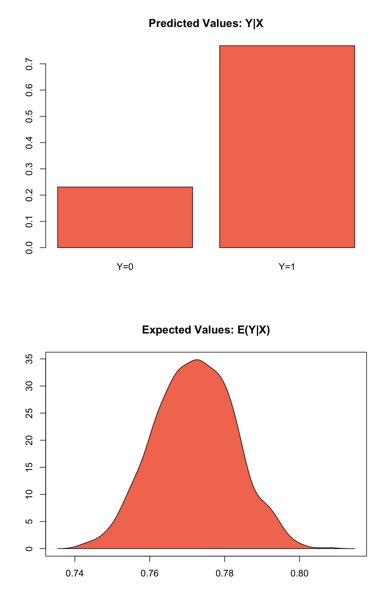
Graphs of Quantities of Interest for Zelig-probit
Model
Let \(Y_i\) be the observed binary dependent variable for observation \(i\) which takes the value of either 0 or 1.
- The stochastic component is given by
\[ Y_i \; \sim \; \textrm{Bernoulli}(\pi_i), \]
where \(\pi_i=\Pr(Y_i=1)\).
- The systematic component is
\[ \pi_i \; = \; \Phi (x_i \beta) \]
where \(\Phi(\mu)\) is the cumulative distribution function of the Normal distribution with mean 0 and unit variance.
Quantities of Interest
- The expected value (qi$ev) is a simulation of predicted probability of success
\[ E(Y) = \pi_i = \Phi(x_i \beta), \]
given a draw of \(\beta\) from its sampling distribution.
The predicted value (qi$pr) is a draw from a Bernoulli distribution with mean \(\pi_i\).
The first difference (qi$fd) in expected values is defined as
\[ \textrm{FD} = \Pr(Y = 1 \mid x_1) - \Pr(Y = 1 \mid x). \]
- The risk ratio (qi$rr) is defined as
\[ \textrm{RR} = \Pr(Y = 1 \mid x_1) / \Pr(Y = 1 \mid x). \]
- In conditional prediction models, the average expected treatment effect (att.ev) for the treatment group is
\[ \frac{1}{\sum_{i=1}^n t_i}\sum_{i:t_i=1}^n \left\{ Y_i(t_i=1) - E[Y_i(t_i=0)] \right\}, \]
where \(t_i\) is a binary explanatory variable defining the treatment (\(t_i=1\)) and control (\(t_i=0\)) groups. Variation in the simulations are due to uncertainty in simulating \(E[Y_i(t_i=0)]\), the counterfactual expected value of \(Y_i\) for observations in the treatment group, under the assumption that everything stays the same except that the treatment indicator is switched to \(t_i=0\).
- In conditional prediction models, the average predicted treatment effect (att.pr) for the treatment group is
\[ \frac{1}{\sum_{i=1}^n t_i}\sum_{i:t_i=1}^n \left\{ Y_i(t_i=1) - \widehat{Y_i(t_i=0)} \right\}, \]
where \(t_i\) is a binary explanatory variable defining the treatment (\(t_i=1\)) and control (\(t_i=0\)) groups. Variation in the simulations are due to uncertainty in simulating \(\widehat{Y_i(t_i=0)}\), the counterfactual predicted value of \(Y_i\) for observations in the treatment group, under the assumption that everything stays the same except that the treatment indicator is switched to \(t_i=0\).
Output Values
The Zelig object stores fields containing everything needed to rerun the Zelig output, and all the results and simulations as they are generated. In addition to the summary commands demonstrated above, some simply utility functions (known as getters) provide easy access to the raw fields most commonly of use for further investigation.
In the example above z.out$get_coef() returns the estimated coefficients, z.out$get_vcov() returns the estimated covariance matrix, and z.out$get_predict() provides predicted values for all observations in the dataset from the analysis.
See also
The probit model is part of the stats package by the R Core Team. Advanced users may wish to refer to help(glm) and help(family).
R Core Team (2017). R: A Language and Environment for Statistical Computing. R Foundation for Statistical Computing, Vienna, Austria. <URL: https://www.R-project.org/>.