Mutlinomial Logit

Built using Zelig version 5.1.4.90000

Multinomial Logistic Regression for Dependent Variables with Unordered Categorical Values with mlogit in ZeligChoice.

Use the multinomial logit distribution to model unordered categorical variables. The dependent variable may be in the format of either character strings or integer values. See Multinomial Bayesian Logistic Regression for a Bayesian version of this model.

Syntax

First load packages:

library(zeligverse)

z.out <- zelig(as.factor(Y) ~ X1 + X23,
               model = "mlogit", data = mydata)
x.out <- setx(z.out)
s.out <- sim(z.out, x = x.out, x1 = NULL)

where Y above is supposed to be a factor variable with levels apples,bananas,oranges. By default, oranges is the last level and omitted. (You cannot specify a different base level at this time.) For $J$ equations, there must be $J + 1$ levels.

Examples

Load the sample data:

data(mexico)

Estimate the empirical model:

z.out1 <- zelig(as.factor(vote88) ~ pristr + othcok + othsocok,
                model = "mlogit", data = mexico, cite = FALSE)

Summarize estimated paramters:

summary(z.out1)

## Model: 
## 
## Call:
## z5$zelig(formula = as.factor(vote88) ~ pristr + othcok + othsocok, 
##     data = mexico)
## 
## 
## Pearson residuals:
##                       Min      1Q  Median      3Q   Max
## log(mu[,1]/mu[,3]) -4.296 -0.6875  0.2791  0.7019 2.102
## log(mu[,2]/mu[,3]) -2.245 -0.4690 -0.2078 -0.0887 4.540
## 
## Coefficients: 
##               Estimate Std. Error z value Pr(>|z|)
## (Intercept):1  2.87082    0.39638   7.243 4.40e-13
## (Intercept):2  0.39915    0.47013   0.849   0.3959
## pristr:1       0.59688    0.09124   6.542 6.07e-11
## pristr:2      -0.12503    0.10428  -1.199   0.2305
## othcok:1      -1.24259    0.11236 -11.059  < 2e-16
## othcok:2      -0.14066    0.13302  -1.057   0.2903
## othsocok:1    -0.30260    0.14960  -2.023   0.0431
## othsocok:2     0.04975    0.16097   0.309   0.7572
## 
## Number of linear predictors:  2 
## 
## Names of linear predictors: log(mu[,1]/mu[,3]), log(mu[,2]/mu[,3])
## 
## Residual deviance: 2360.571 on 2710 degrees of freedom
## 
## Log-likelihood: -1180.286 on 2710 degrees of freedom
## 
## Number of iterations: 4 
## 
## Reference group is level  3  of the response
## Next step: Use 'setx' method

Set the explanatory variables to their default values, with $pristr$ (for the strength of the PRI) equal to 1 (weak) in the baseline values, and equal to 3 (strong) in the alternative values:

x.weak <- setx(z.out1, pristr = 1)
x.strong <- setx(z.out1, pristr = 3)

Generate simulated predicted probabilities qi$ev and differences in the predicted probabilities qi$fd:

s.out.mlogit <- sim(z.out1, x = x.strong, x1 = x.weak)
summary(s.out.mlogit)

## 
##  sim x :
##  -----
## ev
##              mean         sd       50%      2.5%     97.5%
## Pr(Y=1) 0.7125607 0.02126999 0.7135892 0.6700842 0.7537237
## Pr(Y=2) 0.1288215 0.01480180 0.1277746 0.1026277 0.1603835
## Pr(Y=3) 0.1586178 0.01644167 0.1583075 0.1286804 0.1927543
## pv
##        1     2     3
## [1,] 0.7 0.137 0.163
## 
##  sim x1 :
##  -----
## ev
##              mean         sd       50%      2.5%     97.5%
## Pr(Y=1) 0.4031843 0.02184860 0.4033209 0.3613922 0.4468739
## Pr(Y=2) 0.3040039 0.02187937 0.3037288 0.2645768 0.3488399
## Pr(Y=3) 0.2928118 0.02102680 0.2918071 0.2537728 0.3357307
## pv
##          1     2     3
## [1,] 0.408 0.283 0.309
## fd
##               mean         sd        50%        2.5%      97.5%
## Pr(Y=1) -0.3093764 0.03330788 -0.3098321 -0.37300500 -0.2447529
## Pr(Y=2)  0.1751824 0.02784848  0.1755189  0.12114315  0.2301688
## Pr(Y=3)  0.1341940 0.02792288  0.1345650  0.08144286  0.1892681

plot(s.out.mlogit)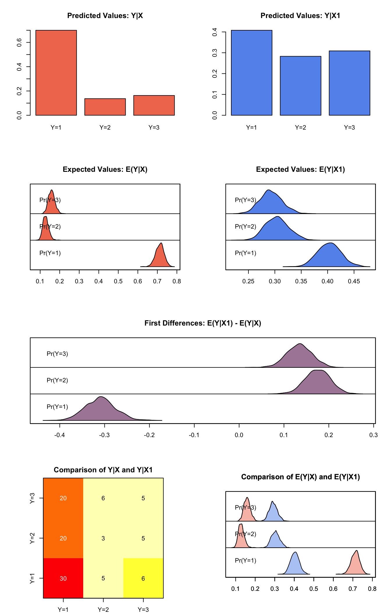

Graphs of Quantities of Interest for Multinomial Logit

Model

Let $Y_i$ be the unordered categorical dependent variable that takes one of the values from 1 to $J$, where $J$ is the total number of categories.

The stochastic component is given by

\[ Y_i \; \sim \; \textrm{Multinomial}(y_{i} \mid \pi_{ij}), \]

where $\pi_{ij}=\Pr(Y_i=j)$ for $j=1,\dots,J$.

The systemic component is given by:

\[ \pi_{ij}\; = \; \frac{\exp(x_{i}\beta_{j})}{\sum^{J}_{k = 1} \exp(x_{i}\beta_{k})}, \]

where $x_i$ is the vector of explanatory variables for observation $i$, and $\beta_j$ is the vector of coefficients for category $j$.

Quantities of Interest

The expected value (qi$ev) is the predicted probability for each category:

\[ E(Y) \; = \; \pi_{ij}\; = \; \frac{\exp(x_{i}\beta_{j})}{\sum^{J}_{k = 1} \exp(x_{i}\beta_{k})}. \]

The predicted value (qi$pr) is a draw from the multinomial distribution defined by the predicted probabilities.
The first difference in predicted probabilities (qi$fd), for each category is given by:

\[ \textrm{FD}_j = \Pr(Y=j \mid x_1) - \Pr(Y=j \mid x) \quad {\rm for} \quad j=1,\dots,J. \]

In conditional prediction models, the average expected treatment effect (att.ev) for the treatment group is

\[ \frac{1}{n_j}\sum_{i:t_i=1}^{n_j} \left\{ Y_i(t_i=1) - E[Y_i(t_i=0)] \right\}, \]

where $t_{i}$ is a binary explanatory variable defining the treatment ($t_{i}=1$) and control ($t_{i}=0$) groups, and $n_j$ is the number of treated observations in category $j$.

In conditional prediction models, the average predicted treatment effect (att.pr) for the treatment group is

\[ \frac{1}{n_j}\sum_{i:t_i=1}^{n_j} \left\{ Y_i(t_i=1) - \widehat{Y_i(t_i=0)} \right\}, \]

where $t_{i}$ is a binary explanatory variable defining the treatment ($t_{i}=1$) and control ($t_{i}=0$) groups, and $n_j$ is the number of treated observations in category $j$.

Output Values

The Zelig object stores fields containing everything needed to rerun the Zelig output, and all the results and simulations as they are generated. In addition to the summary commands demonstrated above, some simply utility functions (known as getters) provide easy access to the raw fields most commonly of use for further investigation.

If the zelig() call output object is z.out, then coef(z.out) returns the estimated coefficients, vcov(z.out) returns the estimated covariance matrix, and predict(z.out) provides predicted values for all observations in the dataset from the analysis.

2017-10-29

Syntax

Examples

Model

Quantities of Interest

Output Values

See also

Contents